


 nueva página del texto (beta)
 Inglés (pdf)
 Artículo en XML
 Referencias del artículo
 Enviar artículo por email
 Citado por SciELO
  Similares en
SciELO
Similares en
SciELO 
 Permalink
Introduction
The calculation of reference crop evapo-transpiration is a key to intelligent irrigation systems. Therefore, accurate estimation of ET0 becomes important in irrigation schedules for planning and optimizing the agriculture area. Numerous methods have been put forward to estimate ET0. Of these, the Penman-Monteith 56 (PM) model has given the best results; it was officially recommended by the Food and Agriculture Organization of the United Nations (FAO) in 1998 (Allen et al., 1998). FAO selected the PM model as the standard equation for ET0 estimation because it can provide the most accurate results in the world. ET0 is also a key parameter in the design of intelligent irrigation for field crops. Engineers need to know the irrigation water consumption requirements for each crop so that they can calculate or estimate the remaining components of the water balance. Also, agriculturists need to obtain the specific water requirements of a crop so that they can generate a satisfactory yield. It is also necessary to know whether these specific requirements are being met with ordinary irrigation.
As described by Kisi (2008) and (Yubin et al., 2014), about 50 measures have been proposed for estimating evapotranspiration, which can be sorted into four types: radiation, temperature, synthetic and evaporating dish. FAO assumed the ET definition given by Smith, Allen and Pereira (1997), and adopted the FAO-56 PM as the sole equation for estimation of ET0.
However, the PM model requires a lot of meteorological data as input, and the calculation process involves complex and nonlinear regression among these factors. So, a simpler and more accurate simulation model needs to seek ET0 in the case of lack of meteorological data. Thus, artificial intelligence algorithms (e.g., neural networks) for reference evapotranspiration (ET0) modeling have been given more attention in recent decades. Feng and Cui (2015) found that an ELM model gave better results than empirical models in the area of central Sichuan. Kisi (2007) estimated daily ET0 using the ANN method and compared their calculation results with the other models. Ozgur Kisiet (2013) proposed a reference evapotranspiration model by LSSVM. Kisi (2011a) considered daily ET0 using wavelet regression model and compared this model to other empirical models. Kisi (2011b) modeled ET0 using evolutionary feed-forward neural networks. Marti, Gonzalez-Altozano and Gasque (2011) used ANN to estimate daily ET0 without local climatic data. Kumar, Raghuwanshi and Singh (2011) researched the application of ANN in estimating evapotranspiration modeling. Shiri et al. (2012) established an ET0 simulation model using GEP (gene expression programming) for Spanish Basque, and found that the GEP model performed better than the ANFIS, Hargreaves and Priestley-Taylor models. Wang, Traore and Kerh (2008), and Traore, Wang and Kerh (2010) estimated daily ET0 using BP-ANN. However, BP-ANN has major disadvantages, such as its slow speed of training and difficulty in selecting parameters. In recent years, new intelligent algorithms have appeared in the industrial field, such as extreme learning machines (ELM) and support vector machine, among others.
In the present study, ELM is proposed as an alternative to other models for predictive control. It can randomly choose hidden nodes and analytically determine the output weights of SLFNs. However, ELM cannot confirm the singularity of the output matrix of the hidden layer, and it also cannot make fine tuning according to the characteristics of the data set, which will affect its efficiency and stability.
The main purpose of this paper is to optimize the ELM approach in the modeling of daily ET0 using the original meteorological data. All previous studies have indicated that intelligent models can input the factors of FAO-56 PM as they estimate ET0. In fact, these factors will be another complex computing project by meteorological raw data, to avoid creating more severe error during multistage formula calculation. Also, the manipulation of the inverse of the matrix is adjusted with reference to the optimal solution and the regularization factor at the same time, which is motivated by the online learning method. In summary, an improved online sequential extreme learning machine (IOS-ELM) is designed, and the new algorithm can produce good generalization performance in a model of daily ET0 in an irrigation system.
Materials and case study
The study was conducted in Yulin (38.27° N, 109.78° E), Ankang (32.72° N, 109.03° E), Hanzhong (33.07°N, 107.7°E) and Xi’an (34.3° N, 108.9° E) in Shaanxi province in China, shown in Fig. 1. The area has a hot and dry climate for the greater part of the year.

Daily meteorological data used for this study was from the years 1971-2014. The following observed eight meteorological variables with daily temporal resolution were used: wind speed at 10m above the ground (Uh), mean temperature (T), mean relative humidity (RH), minimum temperature (Tmin), maximum temperature (Tmax), actual Sunshine duration (n), latitude (φ) and elevation (Z), which were downloaded from China meteorological data sharing service system (http://cdc.nmic.cn/ home.do). Data from the first 29 years (1971-1999) was used to train the models. Data from the next ten years (2000-2009) was used for the test. The data from the remaining years was used for validation. It must be noted, however, that missing data was replaced by the average of the data from the day before and the day before. The regional climate characteristics are given in table 1.

Methodology
Calculation models of reference crop evapotranspiration
The study focused on the comparison of the proposed IOS-ELM model with the ELM, LSSVM, Hargreaves, Mc-Cloud, and Priestley-Taylor models. First, the ET0 values of four cities were calculated using the FAO-56 PM. Then, the standard formula evapotranspiration calculation for all empirical models is shown.
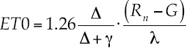
(1) FAO-56 Penman-Monteith:
 (1)
(1)
The original meteorological data of Tmax, T, Tmin, n, Uh, RHm, φ and Z were used in the model:
(2) Hargreaves:
 (2)
(2)
Tmax, T, Tmin, n and φ were used in the model:
(3) Mc-Cloud:
 (3)
(3)
Only T was referred to in the model:
(4) Priestley-Taylor
 (4)
(4)
Tmax, T, Tmin, n and φ were used.
However, these variables are obtained directly or indirectly from the meteorological raw data (Uh, T, RH, Tmin, Tmax, n, φ and Z). Furthermore, the calculation formula for them did not have a precise formula by estimation or experience.
Therefore, the inputs Uh, T, RH, Tmin, Tmax, n, φ and Z, the ET0 output were calculated by the FAO-56 PM method and used for the calibration of the IOS-ELM models. The mean absolute error (MAE), the root mean square error (RMSE), effectiveness index of the model (EF) and self-correlation coefficient (R2) statistics were used for the assessment criteria of the models in this study. EF model efficiency mainly depends on the Nash coefficient EF values; as the values approach one, the efficiency of the model increases. The study adopted the calculation model of the validity index for EF by Nash and Sutcliffe.
Extreme learning machine (ELM)
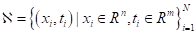
For N random distinct samples (xi, ti) where xi = [xi1, xi2,..., xin]T ∈Rn, ti = [ti1, ti2,..., tin]T ∈Rm and for the standard SLFNs ( Ñ hidden nodes), the activation function g(x) is expressed as:
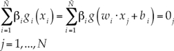 (5)
(5)
where wi = [wi1, wi2,..., win]T is the weight vector connecting the ith hidden node and the input nodes, βi = [βi1, βi2,..., βin]T is the weight vector connecting the ith hidden node and the output nodes and bi is the threshold of the ith hidden node.
 (6)
(6)
The above N equations can be written compactly as
 (7)
(7)
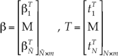
where
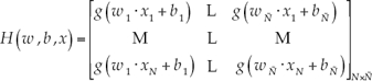 (8)
(8)
 (9)
(9)
where H is called the hidden layer output matrix in the neural network, and the ith column of H is the ith hidden node output toward inputs x1, x2,..., xN.
The aim is to solve the above issues and put forward an extreme learning machine for SLFNs.
A training set was provided as:
 , the activation function g(x), and hidden node number Ñ.
Step 1: Randomly allocate input weight wi and bias bi, i = 1, 2,..., Ñ.
Step 2: Calculate the hidden layer output matrix H.
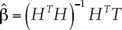
Step 3: Calculate the output weight β.
 (10)
(10)
where T = [t1, ..., tN]T, H+ is a generalized inverse of MP.
Online sequential ELM (OS-ELM)
ELM is a relatively effective and simple algorithm that is also able to learn quickly and generalize well. However, meteorological data are difficult to collect and the data set is large, which may cause a decline in the performance of the ET0 model. Thus, the online sequential extreme learning machine (OS-ELM) by Liang (2006) was referenced in the previous research.
The output weight matrix  is a least-squares solution of (7). Meanwhile, the matter where rank(H) = Ñ the number of hidden nodes (Ao, Xiao, & Mao, 2009) is considered. So, H+ of (10) is given as:
 (11)
(11)
If HT H tends to become fantastic, it can also be made nonsingular by increasing the number of data or choosing a smaller network size. Substituting (11) into (10) gives:
 (12)
(12)
Equation (12) is called the least-squares solution to Hβ = T. Sequential implementation of the least-squares solution of (12) gives the OS-ELM. However, the OS-ELM may have some deficiencies, especially the fact that solving the generalized inverse matrix MP of H may cost a huge amount of time in the training process. The general method of singular value decomposition is used to solve matrix H, but its computational complexity is O(4NÑ2 + 8Ñ3) (Brown, 2009).
Improved algorithm of OS-ELM (IOS-ELM)
This paper proposes an improved OS - ELM called IOS-ELM. This new model was developed by modifying and improving the singularity of the matrix. First, Equation Hβ = T will be replaced by HTHβ = HTT, which has at least one optimization solution. This reduces the computational complexity of solving the inverse, which results in a reduction of the training time. Second, the regular factor l/λ is joined when calculating the output weights. Last, the subsequent online learning stage is added. In theory, this algorithm can provide good generalization performance at an extremely fast learning speed.
Step (1): Allocate random input weights wi and bias bi, initialize network and calculate the initially hidden layer output matrix H0.
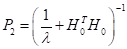
Step (2): Set r = rank(H), if r = N0, then calculate the initial weight matrix β0 = P1H0TT0.If r = N then calculate the initial weight β0 = H0TP2T0.
Where  ,
, 
If r ≠ N0 and r ≠ Ñ, to solve the two optimization models:

Then, the optimization solution B* and β0 can be obtained.
Where  ,
,  ,
,  g is a positive definite symmetric matrix.
Step (3) Set K = 0; then, present the (K + 1)th chunk of new observations:

where NK+1 is the number of observations in the (K + 1)th chunk.
Step (4) Calculate the partially hidden layer output matrix HK+1 for the (K + 1)th chunk of data  , as shown in (17):
 (13)
(13)
Step (5) According to step (1), calculate the output weight βK + 1.
Step (6) Set k = k + 1. Go to Step (3).
Application and results
IOS-ELM model under lack of data
The original eight meteorological parameters chose and combined with a different pattern in this section, which was taken as input values. Meanwhile, the calculation of FAO 56 Penman-Montieth was put as the output value. By this method, the IOS-ELM model is established. However, it needs to further consider the effectiveness of the combination pattern among the eight meteorological data. Therefore, the correlation between ET0 and the data was analyzed. In this way, ISO-ELM can choose reasonable meteorological parameters to complete the forecast even if there is a lack of meteorological data. This is shown in table 4.
It can be clearly seen from table 2 that the ET0 outperformed all eight meteorological parameters in terms of correlation. Although the data set is not similar for different cities, the correlation behaved in the same way. Tmax is closely correlated with evapotranspiration for each city, followed by the average temperature, minimum temperature, the actual sunshine time and wind speed. The influence of the latitude and altitude were so small that they were negligible. Finally, the humidity is negative.

The simulation accuracy of the IOS-ELM model was discussed by referring to table 2 under lack of meteorological data. It should be noted that the latitude and altitude were eliminated because they had virtually no effect on the results. Taking Yulin city as an example, the first 10-year (1971-1999) span of data was used to train the models. Then, using different combinations, the error was analyzed, as well as the correlation coefficient and effectiveness of the prediction. This is shown in table 3.
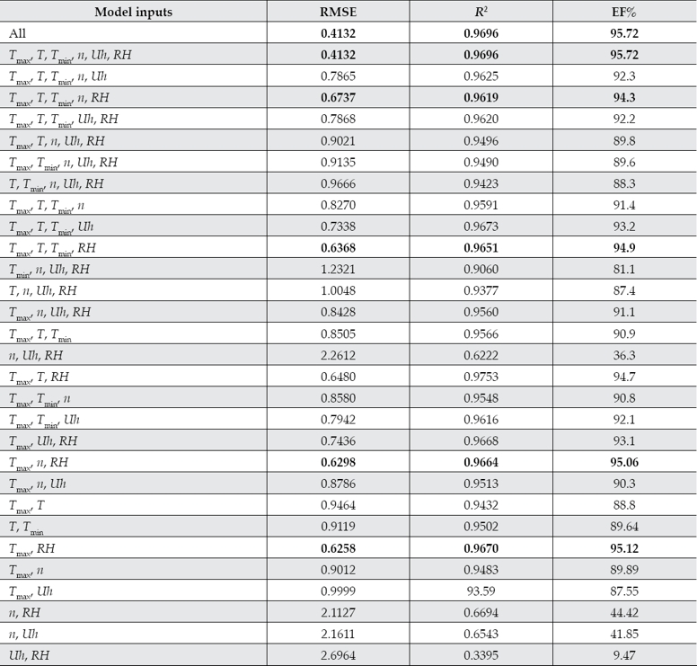

The ISO-ELM model was applied by comparing the different parameters shown in table 3. It is immediately noticeable that the prediction results were the same for eight-parameter and six-parameter inputs. That is because the latitude and altitude almost have no effect on the prediction for the same station. Secondly, the temperature had the largest influence on the prediction, particularly the maximum temperature. As long as the temperature is one of the parameters, the model is accurate. Thirdly, when only two temperatures were used as the inputs, it still performed better than RMSE, EF and R2 statistics. So, properly reducing some variables and adopting reasonable combinations of variables can improve the accuracy of prediction.
Comparison with other calculation formulas
The IOS-ELM model was compared with the ELM and LSSVM, as well as conventional models including Hargreaves, Mc-Cloud and Priestley-Taylor methods in respect of RMSE and MAE statistics in different cities in tables 4-5. There are six parameters as input variables in the model.
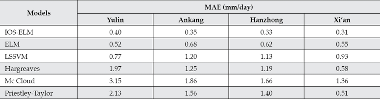
Tables 4-5 show that IOS-ELM outperformed all other models by all performance criteria. Compared with the intelligent and empirical models, the ISO-ELM performed the best value of RMSE<0.46 and MAE<0.41, and the ELM and LSSVM models performed better than the others. A few differences appeared among the Mc Cloud and Priestley-Taylor models. It was also discovered that the Hargreaves method provided better accuracy than other methods among the empirical models.
Although IOS-ELM, ELM and LSSVM models had better simulation effects, the running time is distinguishing, as shown in table 6.

It is clear from table 6 that the IOS-ELM model runs faster than ELM and LSSVM in the process of calculating by at least 24.8%.
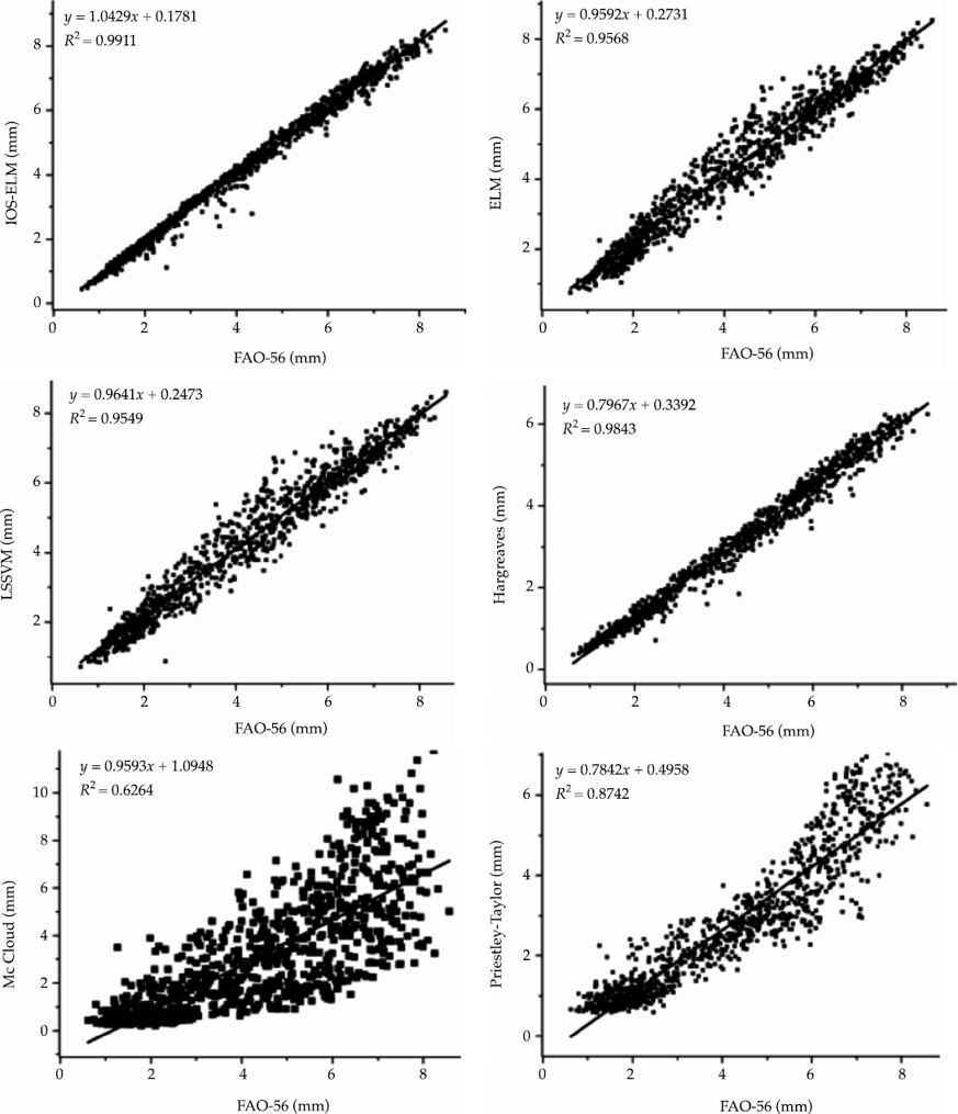
In order to consider the portability and error causes of the IOS - ELM model, the estimates of each model for four cities are shown in figures 2-5 (3, 4) in the form of scatter plots in the validation period. It is generally clear from the scatter plots that the six input ISO-ELM estimates are closer to the corresponding FAO-56 PM ET0 values than other models. The fit line equations y = ax + b and R2 values indicate that the ISO-ELM model performed with better accuracy. Meanwhile, the a and b coefficients of the six-input ISO-ELM model were closer to 1 and 0, respectively, with a higher R2 value than those of the other models.

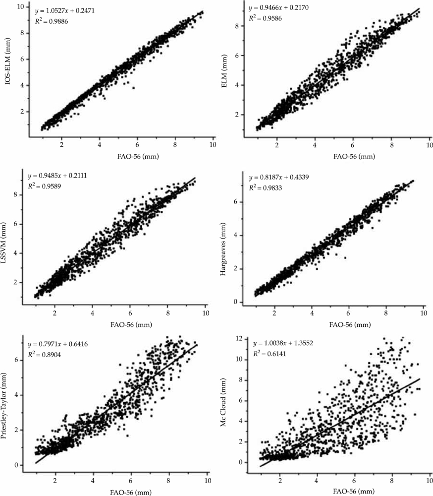

For Yulin, ISO-ELM and ELM estimates were closer to the FAO-56 PM ET0 values than those of the other models (R2 > 0.96). A slight difference exists between LSSVM, and Hargreaves was better than the surplus models. The Mc Cloud estimate had the least accuracy. It can be concluded that the ISO-ELM and ELM models are the best methods to use for daily ET0 estimation in Yulin.
For Ankang, ISO-ELM and Hargreaves were closer to the FAO-56 PM ET0 values, a slight difference exists between LSSVM, and ELM was better than the Mc Cloud model. In this city, the Mc Cloud estimate was also the least accurate (R2 = 0.6141). This leads to the conclusion that in this city, the ISO-ELM and empirical Hargreaves models were the best.
For Hanzhong, ISO-ELM was closer to the FAO-56 PM ET0 of R2 = 0.9911, followed by the Hargreaves, ELM, and LSSVM models. The Mc Cloud and Priestley-Taylor estimates were the least accurate.
For Hanzhong, ISO-ELM was closer to the FAO-56 PM ET0 with R2 = 0.9905, followed by the ELM, LSSVM, Priestley-Taylor, Hargreaves and Mc Cloud models, which had R2 values of 0.9547, 0.9488, 0.8804, 0.8335 and 0.5577, respectively.
The total ET0 estimation of every model is compared in table 7 because of its importance in irrigation management. The ISO-ELM clearly performed better than the other models from the relative error, which was 4.76, 0.23, 0.02 and 0.54%, respectively. In four of the cities, it gave the closest estimate to the total FAO-56 PM ET0 during the validation period.

For Yulin, the ELM and LSSVM had the same accuracy, which was the second best, and had 5274 and 5488 estimates lower than the 10% error, respectively. They were followed by Hargreaves, Priestley-Taylor and, lastly, McCloud (1955), which had the highest error at 64.60%. For Ankang, the LSSVM was ranked as the second best, followed by the ELM, Mc Cloud, Hargreaves and, finally, Priestley-Taylor. For Hangzhong, the LSSVM was ranked as the second best, followed by ELM, Hargreaves, Mc Cloud, and Priestley-Taylor, which had 28.49, 30.37 and 33.50% error, respectively. For Xi’an, the ELM, LSSVM, and Hargreaves were ranked the second best, followed Priestley-Taylor and, finally, Mc Cloud.
In short, for the different cities, the ISO-ELM performed better than the other models, and the other models had different degrees to adapt to the application.
Conclusion
The improved sequential extreme learning machine (IOS-ELM) is designed and applied for simulation of daily reference evapotranspiration through different manipulation of the inverse of the matrix and using the regularization factor and online learning method at the same time Experimental results demonstrated that the IOS-ELM can learn faster and achieve better performance than traditional ELM.
First, the IOS-ELM model effectively overcomes the defects of traditional ELM, such as slow training speed, difficult parameter decisions, difficulty in setting the singularity and effect of data samples.
Second, the potential of the ISO-ELM technique for the estimation of reference evapotranspiration was investigated for four areas in Shaanxi of China; particularly, eight meteorological data were used as inputs.
Third, it was demonstrated that intelligent algorithm models (IOS-ELM, ELM, and LSSVM) are widely applicable to different areas, but empirical models were limited to specific regions and required modification.
Fourth, in the different meteorological data combinations for ET0 estimation, as long as there was a temperature-related parameter calculation, the calculation accuracy of ET0 was over 94%, and Tmax was especially effective. These accurate calculations can be a valuable reference for the development of intelligent irrigation in water decision-making systems.
Notation
The following symbols are used in this paper:
ET0 |
reference evapotranspiration (mm day-1) |
Δ |
slope of the saturation vapor pressure function (kPaC-1) |
Rn |
net radiation (MJ m-2 day-1) |
G |
soil heat flux density (MJ m-2 day-1) |
c |
psychometric constant (kPa C-1) |
T |
mean air temperature (°C) |
U2 |
average24-h wind speed at 2 m height (ms-1) |
Rs |
solar radiation (MJ m-2 day-1) |
es |
the saturation vapor pressure (kPa) |
ea |
the actual vapor pressure (kPa) |

