


 nueva página del texto (beta)
 Inglés (pdf)
 Artículo en XML
 Referencias del artículo
 Enviar artículo por email
 Citado por SciELO
  Similares en
SciELO
Similares en
SciELO 
 Permalink
Introduction
With an analysis by overtopping of the diversion works of Aguamilpa Dam, in Mexico, on January 1992, Marengo-Mogollón (2006) concludes that: "the overtopping event would have been avoided if a hydraulic concrete lining would have been built at the floor, and shotcrete at the walls and vault of the tunnels with vault type (16 x 16 m) section (composite roughness concept) even though the peak inflow rate exceeded by 50% the original design value". This paper shows the analysis made in a hydraulic model with composite roughness that simulates permanent flow in tunnels working as full pipe. While the flow in prototype is mainly governed by gravity, in the model it is also influenced by viscosity nevertheless, working within a limited range of variation of the Reynolds number, and adopting Froude's similitude, has made possible to ignore such influence in all the analyzed models. The main objective of this paper is to validate the theoretical analysis made by Elfman (1993), Marengo-Mogollón (2005) and to prove the best criteria within five formulas that permit the estimation of the roughness coefficient. This paper is organized as follows: first, a brief description of the experimental apparatus is made, then is showed a brief hydraulics review of flow resistance equations, the hydraulic theoretical development in order to evaluate the composite roughness is presented, and the paper concludes by comparing the hydraulic experimental results of the Colebrook equation with the 13 criteria in the transition zone.
Experimental Apparatus
The experimental apparatus is shown in Figure 1. The test section is 0,133 x 0,133 m, and has variable slope with a 9m length. The inlet geometries tested in the model and built in prototype, are rounded. The testes were made with each material acrylic, sandpaper, plastic and carpet (Figure 2), in order to know the main hydraulic proper-ties in each one of them. It was then tested a tunnel of compound roughness that was obtained when it was used the acrylic in the bottom, sandpaper, plastic and carpet in the walls and vault respectively in each one of them. In the analysis, it was considered that Froude's similitude law is applicable, considering that, the friction factor is independent of Reynolds' number.


Resistance and Roughness Coefficients
Leopardi (2004) stated that the tractive force τ produced by the current flow between two sections is proportional to energy gradient,
τ = γRI (1)
At turbulent flow state, τ depends on density ρ (ρ = γ/g) mean velocity V, hydraulic radius R and the roughness K, that is:
Which, using Buckingham's theorem, can be expresses as:
Substituting (3) in (1) makes therefore possible to express the energy gradient as:
The head loss between two sections can be calculated by solving numerically the momentum equation (dh/ds) + Δ = 0, where H is the trinomial of Bernoulli. Therefore, between two sections the following relation holds:
where the index 1 and 2 specify the considered section.
In order to determine the hydraulic gradient along the tunnels, piezometers were installed in the sections 6D and 28D of the models (L1-2 = 3 127 m). According to the entrance records upstream from section, 6D there are strong effects of contraction and in all the experiments, downstream from section 28D there is a clear effect of air entrance; from this section, most of the hypotheses made for the hydraulic functioning as full pipe are no longer valid.
From equation (3):
Using the above relations makes it actually to calculate I, τ, λ, for different values of dis-charge in each model.
Also is calculated the absolute roughness with Colebrook-White criteria; for Re > 25,000 the Colebrook-White (Yen, 2002) relation in the transition zone is often used,
 (7)
(7)
For full circular pipe Colebrook (1939), K
1 = 2.00, K2
= 14.83, K
3 = 2.52, where

And
Then (Eq. (7)) for vault type sections stays:
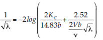 (8)
(8)
Eq. (8) will be used in the analysis.
Hydraulic Models
Models with One Material
Table 1 summarizes the hydraulic parameters calculated for acrylic tunnel model (slopes A1-0.0007, A2-0.001, A3-0.004), for each one, it is re-ported the slope, the flow rate Q (that was tested in the range 0.01 < Q < 0.025 m3/s), the mean velocity V = Q/A, the Reynolds number Re in the range 8 × 10⁴ < Re < 2.4 x 10⁵ (with kinematic viscosity of water v = 0.000001 m2/s), then is calculated for each case I, τ, λ, and the absolute roughness Kb for each criteria (Kb N Nikuardse, K bH Haland, K bCH Churchill and K bSw Swamee, see Table A.1), that is used like bottom roughness in the analysis.

Table 2 shows the hydraulic parameters for sand paper (slopes S1 - 0.001, S2 - 0.004, S3 - 0.008), Table 3 for plastic (slopes P1 - 0.001, P2 - 0.004, P3 - 0.008) and Table 4 for carpet (slopes C1 - 0.001, C2 - 0.004, C3 - 0.008).


For each model, they are reported the same parameters of Table 1 and the absolute roughness measured with Colebrook-White formula; KmC,i means absolute roughness measured in each material (KmC,S sandpaper, KmC,P plastic, KmC,C carpet).
Models with composite roughness
Table 5 shows the hydraulic properties of acrylic-sand paper measured in two roughness model (slopes AS1 - 0.001, AS2 - 0.004, AS -0.008), Table 6, acrylic-plastic (slopes AP1 - 0.001, AP2 - 0.004, AP3 - 0.008), and Table 7, acrylic carpet slopes (AC1 - 0.001, AC2 - 0.004, AC3 - 0. 008). For each model, it's calculated like before I, τ, λ, and the measured absolute roughness KmC,i . calculated with Colebrook-White criteria (KmC,AS is measured for acrylic-sandpaper, KmC,AP for acrylic plastic and KmC,AC acrylic-carpet). In general, this calculus is taken like the "true value" in the transition zone and it is used for comparison in all over analysis.


Composite Roughness Theoretical Development
In an analysis of Head Loses in Tunnels with two roughness (Elfman, 1993) used Nikuradse Equations; in this article, are used other roughness criteria like Haland, Churchill, and Swamee; also are considered the (16) Eqs. Criteria proposed by Yen (2002) for the analysis of acrylic-plastic and acrylic-carpet (the Reynolds number are very high and turbulence is fully developed).
A tunnel that works with composite roughness is shown in Figure 4; has a length L with a cross section that is divided into the corresponding areas Ab and Aw delimited by the perimeters Pb and Pw, has the point of maximum velocity at mid part of tunnel "c" and the contours of equal velocity intersect themselves at right angles.

It is considered that there are two types of roughness Kb (absolute roughness size grain material) at the bottom and Kw in the walls and vault. Total shear force F acting along the tunnel surfaces is equal to the sum of shear force at the bottom (Fb = LPh τ h) and shear force at walls and vault (F w = LPb τ b ); like F = Fb + Fw :
=>LPτ = LPb τ b + LPw τ w (9)
Considering
 (10)
(10)
 (11)
(11)Maximum velocity V max (point "c", Figure 4) is equal to maximum velocity V max b, of the tunnel bottom and the maximum velocity at walls and vault Vmax w :
V max = V max b = V max w (12)
From Nikuradse (1933) analysis:
 (13)
(13)
For the experimental analysis, form Eq. (12) and (13) in Eq. (11):
 (14)
(14)
Head losses at the bottom are equal to those at the walls and vault:
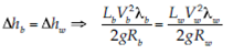 (15)
(15)
 (16)
(16)
Like: 
 (17)
(17)
There are two scenarios of analysis:
Scenario I. If the total roughness factor λ is experimentally known, and also the material of the tunnel bottom Kb, form Eq. (17):
 (18)
(18)
In Eq. (11):
 (19)
(19)
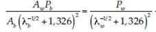
Since A = Ab +Aw:
 (20)
(20)
Tables 8, 9 , 10 and 11 summarizes the calculus of the variables showed in this first scenario Ab , Aw , λ b , λ w , Kw,i ; Kw,i means the absolute roughness in walls and vault (i, is N for Nikuradse, H for Haland, Ch for Churchill and S for Swamee).


Like first comparison, Kw,i calculated with Nikuradse, Haland, Churchill and Swamee criteria is compared with measured sandpaper model (Figure 5). In general the data fits very well the behavior of measured values (Table 3), and calculated values (Tables 8, 9, 10, and 11).
Scenario II. If geometry, absolute roughness materials (Kb , Kw) and influence perimeters (Pb , Pw ) are known, it is desired to calculate total roughness factor λ of the model tunnel.
The absolute roughness values Kw,i calculated in Scenario I (tables 8, 9, 10 and 11) are used in order to calculate λ and the value of KpredC,i with Eq. (17) (and Eq. 14). This predicted values of absolute roughness calculated with Colebrook's formula, let us to compare the measured values (Tables 5, 6, 7 and the predicted values with the theoretical formulation).
Table 12 show the results for Nikuradse, Table 13 for Haland, Table 14 for Churchill and Table 15 for Swamee criteria, using the results obtained from scenario I.


Statistical Comparison
The statistical comparison of any friction factor equation with the Colebrook's equation can be done with the following procedure.
Calculate the friction factor Kpred,i by the criteria selected (Nikradse, Haland, Churchill, Swamee).
Calculate the friction factor value KmC,i measured with the Colebrook's equation.
Calculate the following parameters:
Mean relative error
 (21)
(21)
Maximal positive error
 (22)
(22)
Maximal negative error
 (23)
(23)
Correlation ratio
 (24)
(24)
Standard deviation
 (25)
(25)
Mean variation
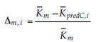 (26)
(26)
Where  is the average value of KmC,i
for the complete set of values:
is the average value of KmC,i
for the complete set of values:
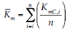 (27)
(27)
In the Table 16 is made a comparison with the mean relative, maximal positive, maximal negative and mean variation error for each criteria (Nikuradse, Haland, Churchill, and Swamee).

The maximal positive relative error maxRE+ = 0.0936 is for Swamee criteria; the maximum negative error belongs to the Nikuradse criteria maxRE - = 0.144.
In Table 20 is shown a summary of this calculus; in which are shown the correlation ratio, standard deviation and mean variation of the error.
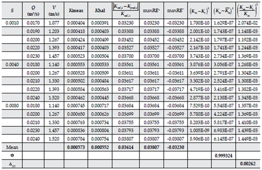


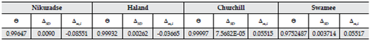
The statistical analysis, show that the best correlation ratio and the minimum standard deviation is for Churchill criteria.
The minimum difference in the in the mean value
Conclusions
It was proposed the Eq. (8) that is a Colebrook-White form, and let to determine the absolute roughness in this kind of tunnels geometries; even when it is applied to the composite roughness. In addition, it was reviewed other equations like Nikuradse, Haland, Churchill and Swamee.
Elfman's (1993) and Marengo-Mogollón (2005) theoretical analysis was reviewed and was proposed two Scenario's analysis. They were compare with models measurements and they were validate. When comparing the results obtained from simple equations with those determined from the experiments their validity is demonstrated to calculate coefficients λ b , λ w and Kw (Scenario I), and λ b , λ w, λ C and KmC,i. in Scenario II. The theoretical development is quite acceptable.
Theoretical model can be applied in model development with this kind of analysis.
In future research, will be possible to analyze the hydraulic behavior in tunnels having other geometries (horseshoe and circular cross sections with composite roughness), so as to be able to define the behavior of the tunnels when functioning as open channels.
It will be possible to validate the equations proposed for the composite roughness with their respective geometries, and to investigate the behavior of the equal-velocity curves with tunnels operating as full pipes.
It should be made special mention in order to measure in prototype tunnels and compare with the results obtained in hydraulic models.
With respect to the statistical analysis, standard deviation (Δ SD ), correlation ratio (Θ), and maximal relative errors (maxRE +), are quite low.
The minimum values of standard deviation Δ SD = 7.58 belongs to Churchill criteria besides the best correlation ratio Θ = 0.9999682. The maximal relative error belongs to Swamee maxRE+ = 0.0936 and the maximum negative error belongs to the Nikuradse criteria maxRE- = 0.144.
The minimum difference in the mean value
Under this analysis it is possible to say that the best theoretical criteria in order to obtain an accurate behavior is with Churchill criteria that offers the best correlation ratio, followed by Haland, Nikuradse and Swamee.
If it is selected standard, division also is Churchill criteria. If mean criteria is selected, Haland gives the best approximation.
The results obtained with Haland criteria are very good also.
Notation
A = cross sectional area.
A = height of triangle defining the area of influence of the floor material in tunnels with composite roughness.
Aw and Aw = areas of influence of the material for the floor slab and for walls and vault, respectively.
d = depth of water at tunnel entrance.
D: pipe diameter.
d/D = ratio between inlet hydraulic head with respect to the tunnel equivalent diameter. equivalent diameter to the circular cross section.
ƒ = Marchi's shape factor.
F = total shear force.
Fb and Fw = shear forces at floor, and at walls and vault, respectively.
g = acceleration of gravity.
h = lost of energy.
K = absolute roughness of the material of the circular conduit.
Kb and Kw = roughness coefficient at floor and at walls and vault, respectively, in a tunnel with composite roughness.
Kn = conversion factor of units for Manning's formula.
Ks = equivalent absolute roughness of the material for non-circular conduits.
l = length of the section.
Le = scale of lines.
LP = area of section under study.
ne = scale of roughness.
P = perimeter.
Q = flow rate.
Qe = scale of flow rates.
Re = Reynolds' number.
Rh = hydraulic radius.
RR = Reynolds' number calculated with the hydraulic radius.
S = hydraulic gradient.
S1 and S2 = slopes of tunnels.
V = mean velocity.
Vb and Vw = mean values at floor, walls and vault.
Ve = scale of velocities.
Vmax = maximum flow velocity.
Vreal = real velocity registered with a Prndtl-Pitot tube.
ρ = density of fluid.
Δ = increment as a percentage.
v = kinematic viscosity of water.
τ = shear stress at the wall.
λ, n, C = coefficients of resistance to flow by Darcy-Weisbach, Manning and Chezy, respectively.
τ b and τ w = shear stresses at perimeter of floor slab and at perimeter of walls and vault, respectively.
λ b and λ w = coefficients of resistance to flow at floor, and at walls and vault, respectively.
λ c = coefficient of resistance calculated with programs developed by Marengo-Mogollón.
Δhb and Δhw = hydraulic head losses at floor and at walls and vault, respectively;
λ m = average coefficient of resistance.


