Artículos técnicos

 

Study of Water Flow in Dams using Successive Over-relaxation

 

Estudio del flujo de agua en presas con sobre relajaciones sucesivas

 

Norma Patricia López-Acosta^* y José León González-Acosta
Universidad Nacional Autónoma de México
*Autor de correspondencia

 

Dirección institucional de los autores

Dra. Norma Patricia López-Acosta

Investigadora
Universidad Nacional Autónoma de México
Instituto de Ingeniería
Circuito Escolar, Ciudad Universitaria, Delegación
Coyoacán
04510 México, D.F., México
Teléfono: +52 (55) 5623 3600, extensión 8555
nlopeza@iingen.unam.mx

M.I. José León González-Acosta

Ingeniero de Proyecto
Universidad Nacional Autónoma de México
Instituto de Ingeniería
Circuito Escolar, Ciudad Universitaria, Delegación
Coyoacán
04510 México, D.F., México
Teléfono: +52 (55) 5623 3600, extensión 8555
lgonzalez.a87@gmail.com

 

Received: 18/06/2014.
Aproved: 10/06/2015.

 

Abstract

Free surface problems represent boundary value problems in which a portion of the boundary, the free surface, is unknown and must be determined as part of the solution. Classical rigorous and approximate procedures used to draw this line are limited to homogeneous and isotropic media with specific geometries. Currently, this can be determined using numerical methods such as the finite element method (FEM). Nevertheless, FEM requires the storing and handling of a large number of matrices to solve linear equation systems, increasing calculation time. The present article proposes an alternative to analyze free surface problems based on the numerical solution of finite difference equations using the successive over-relaxation method (SOR). Two techniques are implemented with the SOR method— Baiocchi's Solution and the Extended Pressure Method with the iterative Gauss-Seidel process. First, the theoretical basis for these methods are provided. Then, their applicability is described according to an analysis of unconfined flow in a homogeneous and a heterogeneous dam. As part of the results, the upper flow lines obtained with each technique and the flow networks calculated with the SOR method are presented and the use of finite difference equations to determine the hydraulic gradient and flow rate through the flow domain is described. Lastly, conclusions and recommendations for applying and optimizing the use of these techniques are provided.

Keywords: Free surface, unconfined flow, Successive Over Relaxation (SOR), Gauss-Seidel's iterative process, finite differences, upper flow line, Extended Pressure method, Baiocchi's method, flow networks in dams.

 

Resumen

Los denominados problemas de superficie libre son problemas de valores de frontera en los que una porción de la frontera, la superficie libre, no se conoce y debe determinarse como parte de la solución. Los procedimientos rigurosos y aproximados clásicos para el trazo de esta línea se limitan a medios homogéneos e isótropos con geometrías particulares. Actualmente es posible emplear métodos numéricos como los elementos finitos (MEF) para su determinación. Sin embargo, el MEF requiere la resolución de sistemas de ecuaciones lineales que involucran el almacenamiento y manejo de un gran número de matrices que incrementan el tiempo de cálculo. En este artículo se propone una alternativa para analizar problemas de superficie libre que se basa en la resolución numérica de ecuaciones de diferencias finitas mediante el método de sobre relajaciones sucesivas (SOR, Successive Overrelaxation). Se expone la implementación de dos técnicas basadas en el método SOR: la Solución de Baiocchi y el Método de la Presión Extendida, aplicando el proceso iterativo de Gauss-Seidel. Inicialmente se proporcionan las bases teóricas de estos métodos. De manera posterior, su aplicabilidad queda expuesta con el análisis del flujo no confinado en una presa homogénea y en otra heterogénea. Como parte de los resultados, se presentan las líneas de flujo superior obtenidas con cada técnica y las redes de flujo calculadas con el método SOR; asimismo, se explica cómo determinar el gradiente hidráulico y el gasto de infiltración a través del dominio de flujo mediante ecuaciones de diferencias finitas. Por último, se proporcionan comentarios concluyentes y recomendaciones de cómo aplicar y optimar el empleo de estas técnicas.

Palabras clave: superficie libre, flujo no confinado, Sobre Relajaciones Sucesivas (SOR), proceso iterativo de Gauss-Seidel, diferencias finitas, línea superior de flujo, Método de la Presión Extendida, método de Baiocchi, redes de flujo en presas.

 

Introduction

The classical relaxation method is an iterative process in which solutions for water flow through porous media can be obtained by simply knowing the domain geometry and hydraulic boundary conditions (Allen, 1954; Finnemore & Perry, 1968). This method can solve Laplace's equation for a point (node) relative to its surrounding points using an algebraic finite difference equation (Southwell, 1940). For this procedure, a square mesh with dimensions of Δ_x= Δ_y is drawn in the flow zone if the medium is homogenous and isotropic, and a rectangular mesh with dimensions of Δ_x ≠ Δ_y is drawn if the medium is anisotropic. The intersections of the squares or rectangles constitute the nodes of the mesh. For these nodes, approximate values of the hydraulic head or potential h (points where h requires to be calculated) must be assigned while respecting the known values of h in the flow boundaries. These values usually correspond to the upper and lower water levels or the upstream water level (UWL) and downstream water level (DWL) of the problem at hand (known as the Dirichlet boundary conditions; Cheng & Cheng, 2005). The values assigned in the nodes are arbitrary and can be zero or the result of a reasonable estimation. However, although there are several techniques that can be used to ensure that the value of the potential imposed on the nodes where h is not known is as accurate as possible (Young, 1950), it is important to verify the precision of the assigned data manually by calculating the residue in each node. For example, the difference between the hydraulic potential of the four surrounding nodes is calculated with regard to the central or interior node, and so on. Therefore, the relaxation procedure involves the systematic refinement of this residue throughout the grid until the residue in all mesh nodes of interest is zero or practically zero. This value indicates compliance with Laplace's equation when expressed as a finite difference and results in a solution for a certain water flow problem (Allen, 1954; Finnemore & Perry, 1968). The classical relaxation method has several disadvantages. For example, this method becomes long and tedious when trying to obtain approximate solutions if the method has not been programmed using a computer. Besides, this method does not provide general solutions and must be applied to a particular case. However, the classical relaxation method can be adapted for diverse conditions. Due to the versatility that is demonstrated for this method, several improvements have been made, including optimization of the calculation time, taking into account the variations of the materials in the flow region, and solving more complex problems, such as free surface problems (unconfined flow).

The Successive Overrelaxation (SOR) method (Young, 1950) is a modification to the classical relaxation method. This method is powerful and can be used to obtain approximate numerical solutions for multiple equations with unknown analytical solutions (Young, 1950). An important advantage of the SOR method is that it automatically solves the variations in the hydraulic potential for all mesh nodes that represents the flow region. The SOR method uses the Gauss-Seidel iterative process, which utilizes cyclic finite difference equations to solve the problem of interest (Wang & Anderson, 1982). Applying this method, the solution process is automatically repeated for each node until the desired tolerance or minimum error is obtained. For unconfined flow problems in which the upper flow line or free surface is unknown a priori, methods have been devised to modify the ruling equations of the nodes. These methods can be used for solving free surface problems with the basics of SOR method, such as the Baiocchi's solution (Baiocchi, 1971; Bruch, 1980) and the Extended Pressure method (Brezis, Kinderlehrer, & Stampacchia, 1978; Bardet & Tobita, 2002). The first solution is useful for homogenous media, and the second solution is useful for homogenous and heterogeneous media. However, these methods have not been applied to practical cases.

Generally, free surface problems represent a challenge in many areas of fluid mechanics because they involve boundary value problems in which a portion of the boundary is unknown and must be determined as part of the solution (Cryer, 1970). The presence of the free surface or water table makes the analysis methods more difficult. Dupuit's parabola (Dupuit, 1863) and Kozeny's parabola (Kozeny, 1931) are rigorous solutions for drawing the upper flow line and are only applicable for homogenous and isotropic media with vertical walls (Dupuit) or with filters (Kozeny). Other approximated methods, such as the tangent (Schaffernak, 1917; Iterson, 1916, 1917) and sine methods (Casagrande, 1932), allow mainly calculate the discharge point of the upper flow line. Currently, numerical methods, such as the finite element methods (FEM), can be used to determine the discharge point of the upper flow line. However, the FEM requires solving a system of linear equations and involves storing and handling matrices that increase the calculation time.

This paper aimed to implement the SOR method as an alternative for analyzing free surface or unconfined flow problems in homogenous and heterogeneous media. First, the theoretical background of water flow in soils is provided, especially the solution to Laplace's equation using finite differences. Next, the basic equations of the SOR method are obtained. Subsequently, this technique is enabled to evaluate unconfined flow problems using the Baiocchi's and Extended Pressure methods. The applicability of these techniques is demonstrated by analyzing the unconfined flow of water through a homogenous earth dam and a dam composed of different materials. We explain how to determine the upper flow line and use its position to solve the flow problem by considering confined flow and modifying the boundary conditions and the fundamental equations to determine the equipotential and flow lines. Thus, the upper flow line is obtained for each technique and the flow nets are calculated with the SOR method. In addition, we explain how to calculate the hydraulic gradient and the seepage flux or flow rate through the flow domain using finite difference equations. Finally, we present concluding remarks and recommendations regarding the application of the SOR method.

 

Theoretical Basis of Water Flow in Soils

Laplace's Equation

The laminar flow through porous media obeys Darcy's law and is governed by the following equation:

where:

v = discharge velocity.

h = total pressure or total hydraulic head.

k = permeability of the soil.

l = distance traveled by a water particle.

In vector format (Harr, 1962):

Furthermore, the total pressure h is defined by the Bernoulli's law as follows (neglecting the velocity head):

where:

p = hydrostatic pressure (or pore pressure).

ρ = water density.

g = acceleration due to gravity.

y = position pressure with respect to a level of reference.

Because the amounts of incoming and outgoing flow in the normal direction n to the faces of a cubic element with dimensions of dx, dy and dz is the same (due to the principle of flow continuity), the following equation holds:

By factoring and removing terms, the continuity equation is obtained in three dimensions as follows:

To solve flow problems, it is convenient to use a velocity potential function φ rather than the total pressure h. The φ is described as follows:

Therefore, the discharge velocity in each of the main directions becomes:

Thus, Laplace's equation is obtained by substituting equation (7) in equation (5):

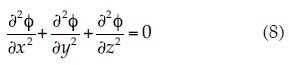
If the medium is homogenous and isotropic and flow only occurs in two dimensions (X and Y, two-dimensional flow), then:

 

Approximate Solution of Laplace's Equation by Means of Finite Differences

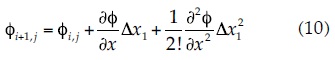
The basic concept of the finite difference method is based on replacing the continuous partial derivatives of the equation that governs water flow with the variation ratio of the x and y variables in small finite increments (Mahmud, 1996). In this way, the following equations are obtained when applying Taylor series expansion to the potential function φ (Mitchell & Griffiths, 1980):

and:

where:

Δx₁ = distance in the X₁ direction between two nodes.

Δx₂ = distance in the X₂ direction between two nodes.

i = row in which the node of interest is located.

j = column in which the node of interest is located.

Figure 1 shows the representation of a node that is affected by four surrounding nodes and can be used to observe the previously mentioned variables.

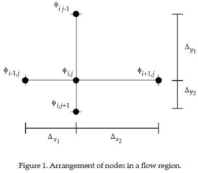
Expression (10) is an approximation to the solution of Laplace's equation regarding the central and the frontal nodes (φ_i+1,j). Equation (11) represents an approximation to the solution of Laplace's equation regarding the central and rear nodes (φ_i+1,j). The equations for the upper (φ_i+1,j) and lower (φ_i+1,j) nodes are analogues to expressions (10) and (11). From equations (10) and (11), and by applying a series of mathematical manipulations, the solution of the potential function φ_i,j is given by:

If then:

Equation (13) approximates the solution of the Laplace's equation by the classical relaxation method in terms of finite differences. From this approximation, the solutions of the nodes located inside the flow region of interest are obtained. Likewise, the expressions for the nodes in other locations (impervious boundaries, corners, etc.) are determined.

 

Basis of the Basic Equations of the SOR Method

From equation (13), it is possible to apply a series of algebraic operations to obtain the basic equations of the successive overrelaxation method by assuming the following (Young, 1950):

where:

c = residue after two Gauss-Seidel iterations in a single node.

m = iteration number.

= value of the potential function in the node i,j in iteration m.

₌ value of the potential function in the same node i,j in iteration m+1.

By solving from (14), the following equation is obtained (Young, 1950):

where α is a relaxation factor that is added to the equation. For fast convergence, it is recommended that the relaxation factor is within the interval of 1 < α< 2 (Young, 1950). In fact, the value of a is used to name this method as follows: over-relaxation if 1 < α< 2, and under-relaxation if 0 < α< 1 (for α > 2 the process diverges). Additionally, if equation (13) is substituted in equations (14) and (15), then (Wang & Anderson, 1982):

Expression (16) represents the solution to Laplace's equation for a central node with respect to the adjacent nodes using the SOR method. The expressions described with this method for evaluating the potential function f (Wang & Anderson, 1982) are applicable to other flow conditions that are discussed in this paper. Thereby, for a node located at the boundary of an impervious horizontal surface, the solution to Laplace's equation with the SOR method is:

For a node located in a vertical impervious boundary, the solution is:

For the nodes located in the vertices or exterior corners, the solution is:

For the nodes located in the transition zone of two materials with different permeability's, the solution is:

For a node located in the transition zone of two materials and at an impervious lower boundary, the solution is:

where γ = k₂/k₁, k₁ is the permeability of the first material and k₂ is the permeability of the second material.

 

Implementing the SOR Method for Problems of Unconfined Water Flow

If the zones of the flow domain where the water pressure is zero are determined for free surface or unconfined flow problems, it is assumed that the upper flow line is defined at these points (Cryer, 1970). The Baiocchi's solution (Baiocchi, 1971; Bruch, 1980) and the Extended Pressure method (Brezis et al., 1978; Bardet & Tobita, 2002) are two variants of the SOR method that can be used to determine the position of the upper flow line in homogenous media or media composed of materials with different permeability values, respectively (as explained below).

 

Solution to the Problems in Homogenous Media Using the Baiocchi's Method (Baiocchi, 1971; Bruch, 1980)

Instead of using the velocity potential function φ, the Baiocchi's method mathematically solves Laplace's equation (in the flow zone and in its boundaries) for unconfined flow by using a new variable w that depends on the geometrical characteristics of the problem (Bruch, 1980). The w variable is numerically expressed with finite difference linear equations for the nodes of the mesh that discretize the flow zone under study. Applying this method, it is possible to determine the position of the upper flow line in a homogenous medium because it generates values of zero (w = 0) for the nodes with a total water pressure of zero (this means that these points are at atmospheric pressure). The form of the expression that describes w depends on the location of the nodes in the mesh. Consequently, the different expressions for obtaining w are described in the following paragraphs (Bruch, 1980). For nodes inside the flow region, w is determined as follows:

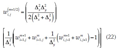
As well:

where α is the relaxation factor, max {...} is the maximum absolute value between the two data values of equation (23), and the remaining variables are defined in the previous sections. For the nodes located in the upstream equipotential boundary, the variable w is defined as:

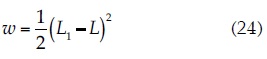
For the node located in the downstream equipotential boundary, w is calculated by:

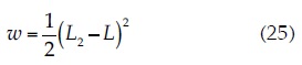
where L₁ is the height of the upstream water level (UWL), L₂ is the height of the downstream water level (DWL), and L is the height from a point of reference (for example, the foundation soil of the dam) to each one of the nodes according to the studied case.

For nodes located in the lower flow boundary (base of the dam), the solution for w is:

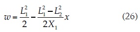
where X₁ represents the length of the base of the dam in X direction, and x is the location of each node in X direction and 0 (origin) is the toe of the dam slope.

 

Solutions to the Problems in Heterogeneous Media Using the ExtendedPressure Method (Brezis et al., 1978; Bardet & Tobita, 2002)

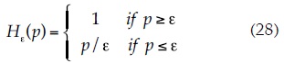
In this method, the hydrostatic pressure p is assumed as the unknown quantity instead of the potential function φ. Moreover, the Extended Pressure concept (Brezis et al., 1978; Bardet & Tobita, 2002) is used, which modifies Darcy's law as follows:

where ε is the separation (Δy) between two nodes in the Y direction. Additionally:

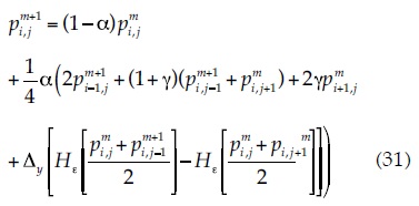
The solution to equation (27) is determined similarly to obtaining the solution of Laplace's equation using the SOR method (equation 16) by introducing the relaxation factor α. Again, the expressions that govern the behavior at each node depend on their locations in the flow domain. Thus, the equations that define p are described below (Bardet & Tobita, 2002). To evaluate the behavior of the nodes located inside the flow region, the hydrostatic pressure p is defined as:

 

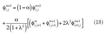
For the nodes located in an impervious lower flow boundary, the hydrostatic pressure is determined as follows:

In contrast to the Baiocchi's method, the value that is assigned to the nodes at the equipotential boundaries of the mesh is equal to the hydrostatic pressure regarding the upstream or downstream water levels (UWL or DWL, respectively) for each specific case when using the Extended Pressure method.

For the nodes located at the transition between two materials with different permeability's, the following expression is used to calculate the pressure:

For a node located in the transition zone and in the impervious lower boundary, the applicable equation is:

where γ = k₂/k₁. Here, k₁ is the permeability of the firstmaterial and k₂ is the permeability of the second material.

 

Practical Applications

The Initial Conditions using the Baiocchi's and Extended Pressure Methods

One advantage of working with equations in the nodes of a mesh is that they can be programmed without major complications using spread sheets without more sophisticated coding or programming in other types of software. The equations of each node are independently and numerically solved by only considering the data of the adjacent nodes. In consequence, it is not necessary (as in the finite element method) to study the behavior of each element, and then with the assembly to solve complex linear equation systems when evaluating global behavior. This process involves handling and storing a large number of matrices. In the following paragraphs, the use of spreadsheets is illustrated by using the equations of the SOR method to solve two free surface (unconfined flow) problems in dams.

Figure 2 shows an unconfined flow problem in a homogenous and isotropic dam. In the same figure, the locations of some of the nodes and boundaries with the equations or conditions that govern their behavior are shown. These parameters are listed in Table 1 for the Baiocchi's and Extended Pressure methods.

Similarly, Figure 3 exemplifies a flow problem in a dam that is constructed of materials with different permeability's. The boundary conditions and their governing equations for this case when applying the Extended Pressure method are provided in Table 2.

It is recommended that the nodes in the downstream slope of the dam or earth structure (boundaries FGH, indicated with open circles in Figure 2 and Figure 3, respectively) should be placed outside the flow zone (the ghost nodes) (Wang & Anderson, 1982). This process allows the upper flowline to develop fully inside the flowzone rather than being forced to end exactly at the DWL (downstream water level). Otherwise, it is possible that the free discharge surface will not be well defined.

In the problems discussed herein, a relaxation factor of α = 1.7 was assumed, which is the recommended value for significantly optimizing and reducing the calculation time (Salmasi & Azamathulla, 2013). Besides, the analyses are conducted in the following stages: 1) calculation of the upper flowline position, 2) evaluation of the potential function φ for drawing up equipotential lines, 3) estimation of the stream function values Ψ for drawing up the flow lines, 4) calculation of the hydraulic gradients, and 5) evaluation of the seepage flux (as described below).

 

Flow Problem Solution for a Homogenous Dam

The flow of water through a homogenous earth dam that was built on impervious rock was studied. Figure 4 shows the geometrical characteristics and the mesh that were used for implementing the SOR method, with a node spacing or distance of Δ_x = Δ_y = 0.20 m. The studied dam has 2:1 slopes upstream and down-stream with assumed water levels of UWL = 9.0 m (upstream) and DWL = 2.0 m (downstream).

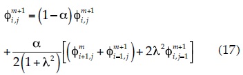
Along with a spreadsheet, Figure 5 presents the results that were obtained in stage 1) when deducing the position of the upper flowline. The spreadsheet was cut so to appreciate the results at the toe of the dam and near its crest (in part of the upstream slope). The values in each of the cells represent the solutions that were obtained by means of the Baiocchi's (Figure 5a) and Extended Pressure (Figure 5b) equations, which are indicated in Section "The initial conditions using the Baiocchi's and Extended Pressure methods".

Once the upper flow line is defined, the boundary conditions are modified for continuing the calculation process. First, the potential function φ is determined for drawing up the equipotential lines. Second, the values of the stream function Ψ are obtained for drawing up the flow lines. In this way, in stage 2), the respective values of total pressure h (Equation (3)) are assigned in the nodes located at the boundaries of water infiltration (upstream), the discharge (downstream) area, and in the upper flow line to evaluate the potential function φ. Whereas, the nodes of the lower flow boundary (impervious base of the dam) are governed by Equation (17). In stage 3) considering an analogy of Ψ with φ, it is possible to use the same equations for calculating the stream function Ψ that were used for calculating the potential function φ. Here, the boundary conditions are modified again according to the following situations: a) in the lower flow line (impervious boundary), a value of zero is assigned to all nodes (Ψ₁ = 0) and b) the value assigned to the upper flow line represents the flux that passes between the upper and lower flow lines, which corresponds to the total seepage flux through the dam (Ψ₂ = q_tot) (Bardet & Tobita, 2002; Bosch & Davis, 1997). Figure 6a exhibits the position of the upper flow line that was obtained using the Baiocchi's and Extended Pressure techniques (based on the SOR method). For comparison purposes, this figure also shows the position of the upper flow line that was calculated with the Kozeny's parabola (a rigorous method proposed by Kozeny in 1931) and the finite element method (an approximate numerical method that was applied here through the SEEP/W algorithm, Geo-Slope International Ltd., 2008).

As revealed in Figure 6a, the upper flow lines calculated with the procedure proposed here using the SOR method were similar to those determined by the other methods. In particular, the Extended Pressure technique matches the solution that was obtained by the finite element method. Figure 6b provides the numerically calculated flow net based on the SOR method, which considers the position of the upper flow line that was obtained with the Extended Pressure method. Additionally, Figure 6b confirms that the SOR method can be used to define the flow net accurately.

 

Flow Problem Solution for a Dam Composed of Materials with Different Permeability's

Here, the water flow through a dam composed of distinct materials was studied. Figure 7 shows the geometric characteristics and the mesh that was used for implementing the SOR method with a node spacing or distance of Δx = 0.20 and Δy = 0.10 m, respectively. Likewise, this figure shows an upstream water level of UWL = 9.0 m (1.0 m below the crest of the dam) and upstream and downstream slopes of 2:1 for the dam. The core of the dam is composed of a low permeability material (k₂) relative to the adjacent transition materials (k₁ and k₃). The ratio between the permeabilities of the core material and the upstream transition material is k₂/k₁ = 0.1, and the ratio between the core material permeabilities and the downstream transition material is k₃/k₂ = 10. At the toe of this dam, a horizontal sand filter with high permeability and a length of 10.0 m was placed, which relieves water pressure to avoid or mitigate erosion problems at this part of the dam.

This practical application is solved similarly to the previous application as follows: stage 1) deduction of the upper flow line position with the Extended Pressure method, stage 2) evaluation of the potential function φ for drawing the equipotentials lines, and stage 3) calculation of the stream function values Ψ for drawing the flow lines. Moreover, once the water pressure variations in the dam are obtained, in order to complete the flow problem solution the hydraulic gradients are determined in stage 4) and the seepage flux is calculated in stage 5) as indicated below. To evaluate the hydraulic gradient (resulting magnitude) inside the flow zone, the following expression can be applied in terms of finite differences (Budhu, 2000):

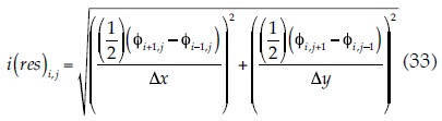
where i(res) is the hydraulic gradient value (resulting magnitude) in each node of the mesh.

The flow rate calculation is determined by drawing a vertical line or plane across the flow region and using the pairs of nodes over this line that are located in transverse direction to the flow. Thus, the flow rate is obtained from the following equation (Budhu, 2000):

where:

q_tot = total flow rate across the flow zone.

k_x = permeability in the X direction.

D = nodes located in the lower line.

E = nodes located in the upper line.

Δx = distance between two nodes in the X direction.

Δy = distance between two nodes in the Y direction.

Figure 8 shows the spreadsheet that is used to solve the problem. The values of the cells correspond with the hydrostatic pressure (p) that was calculated for the nodes of the impervious boundary, the filter and inside the flow zone when applying the Extended Pressure method (the spreadsheet is cut off to show a portion of the results).

Figure 9a shows the flow net that was numerically obtained with the SOR method in the analyzed dam. In this case, the upper flow line was calculated with the Extended Pressure technique. For comparison purposes, Figure 9b presents the upper flow line that was obtained using the finite element method through the SEEP/W algorithm (Geo-Slope International Ltd., 2008). When comparing the results obtained with SOR and FEM, similarities were observed. In the zone of the material with lower permeability, a greater loss of hydraulic head occurs. However, due to the law of continuity for the steady-state flow, the total flow rate that traverses the three flow zones is the same q_tot = 0.65 m³/s. This flow rate was calculated in terms of finite differences with Equation (34). Similarly, the classical theory notes (Cedergren, 1989) cases where the flow domain consists of two or more portions with different permeabilities (each one consists of a homogenous and isotropic soil), in which the flow net is distorted at the boundaries between contiguous materials (Figures 9a and 9b) so that the same amount of flux passes through both sides of the boundary between two flow lines. Thus, Figures 9a and 9b point out that the permeability is lower for the wider flow channels and greater for the narrower flow channels (Flores, 2000).

Finally, Figure 10 provides the hydraulic gradient (resulting magnitude) in the flow zone that was calculated using finite differences with Equation (33).

 

Conclusions

Here, an alternative for analyzing free surface problems was proposed. This alternative was established on the numerical solution of finite difference equations using the SOR (Successive Overrelaxation) method. The implementation of two techniques based on the SOR method were shown, including the Baiocchi's solution and the Extended Pressure method, which utilize the Gauss-Seidel iterative process. The equations of the SOR method can be easily enabled using spreadsheets for the solutions of different types of flow problems of variable complexity (such as free surface problems) without requiring sophisticated programing or specialized software. Using the SOR method, the equations of each node are numerically solved independently and automatically by considering the data of the adjacent nodes. Thus, it is not necessary (as in other numerical methods such as the FEM method) to study the behavior of each element and afterward with the assembly to solve complex systems of linear equations in order to evaluate the global behavior, which involves the storage and handling of a large number of matrices that increase the calculation time. The applicability of the method was exposed by the unconfined water flow analysis through homogenous and heterogeneous earth dams. By using the SOR technique, the variations of the potential function φ and the stream function Ψ were calculated for numerically drawing the flow net. In addition, the resulting magnitude of the hydraulic gradient, the total flow rate and the position of the upper flow line were estimated with the Baiocchi's and Extended Pressure techniques.

From the analyses performed, the Extended Pressure method was shown to provide results with better approximation than the Baiocchi's solution. In particular, the Extended Pressure method provides practically equal results to those calculated with FEM. One additional advantage that was observed in the Extended Pressure method is that it does not require a very refined discretization of the flow domain. In consequence, this method can be used to obtain good results even when the separation between the nodes of the mesh is large (a coarse grid). The obtained results demonstrate that the techniques implemented in this paper are simple and easily applied. Furthermore, these techniques provided similar results to those obtained with the currently popular numerical methods, such as the finite element method.

 

Acknowledgments

The co-author acknowledges the Scholarship Program (Post-Masters level) of the Instituto de Ingeniería of the Universidad Nacional Autónoma de México (UNAM) for providing support during the realization of this paper and the researches related to this subject. It is expected that the developed works significantly contribute to the geotechnical engineering scientific community.

 

References

Allen, N. de G. (1954). Relaxation Methods in Engineering and Science (257 pp.). New York: McGraw Hill.         [ Links ]

Baiocchi, C. (1971). Sur un problème a frontière libre traduisant le filtrage de liquides à travers des milieux poreux (On a Free Surface Problem Considering the Liquid Filtration through Porous Media) (pp. 1215-1217). Paris: C.R. Academie des Sciences 273.         [ Links ]

Bardet, J. P., & Tobita, T. (January, 2002). A Practical Method for Solving Free-Surface Seepage Problems. Computers and Geotechnics, 29, 451-475.         [ Links ]

Bosch, D. D., & Davis, F. M. (June, 1997). Methods for Calculating Flow from Observed or Simulated Hydraulic Head. Advances in Engineering Software, 28, 267-272.         [ Links ]

Brezis, H., Kinderlehrer, D., & Stampacchia, G. (1978). Sur une nouvelle formulation du problème de l'écoulement à travers une digue (On a New Formulation of the Flow Problem through a Dam). Serie A. Paris: C. R. Academie des Sciences.         [ Links ]

Bruch, J. C. (1980). A Survey of Free Boundary Value Problems in the Theory of Fluid Flow through Porous Media: Variation Inequality Approach - Part I. Advances in Water Resources, 3, 65-80.         [ Links ]

Budhu, M. (2000). Soil Mechanics and Foundations (616 pp.). New York: John Wiley & Sons Inc.         [ Links ]

Casagrande, L. (1932). Naeherungsmethoden zur Bestimmung von Art und Menge der Sickerung durch geschuettete Dämme (Approximate Methods to Determine the Seepage through Spillway Dams). Thesis. Vienna: Institute of Technology.         [ Links ]

Cedergren, H. R. (1989) Seepage, Drainage and Flow Nets. New York: John Wiley & Sons.         [ Links ]

Cheng, A., & Cheng, D. T. (2005). Heritage and Early History of the Boundary Element Method. Engineering Analysis with Boundary Elements, 29, 268-302.         [ Links ]

Cryer, C. W. (July 1970). On the Approximate Solution of Free Boundary Problems Using Finite Differences. Journal of the Association for Computing Machinery, 17, 397-411.         [ Links ]

Dupuit, J. (1863). Etudes théoriques et pratiques sur le mouvement des eaux dans les canaux découverts et à travers les terrains perméables (Theoretical and Practical Studies of the Movement of Water in Open Channels through Permeable Media). Paris: Dunond.         [ Links ]

Finnemore, E. J., & Perry, B. (October, 1968). Seepage through an Earth Dam Computed by the Relaxation Technique. Water Resources Research, 4, 1059-1067.         [ Links ]

Flores, R. (2000). Flujo de agua a través de los suelos (4a edición). Avances en Hidráulica 4. México, DF: Asociación Mexicana de Hidráulica, Instituto Mexicano de Tecnología del Agua.         [ Links ]

Geo-Slope International, SEEP/W-2007 (2008). Scientific Manual: Seepage Modeling with SEEP/W 2007. An Engineering Methodology (3rd Ed.). Alberta, Canada: Geo-Slope International, Ldt, Calgary.         [ Links ]

Harr, M. E. (1962). Groundwater and Seepage (313 pp.). New York: McGraw-Hill Inc.         [ Links ]

Iterson, F. F. Th. Van. (1916, 1917). Eenige Theoretische Beschouwinger over Kwel (Some Theoretical Considerations about Seepage). De Ingenieur, 31, 629-633.         [ Links ]

Kozeny, J. (1931). Grundwasserbewegung bei freiem Spiegel, Fluss-und Kanalversickerung- Nasserkraft und Wasserwirtschaft (Groundwater Movement with Free Surface in Channels and Hydroelectric Energy by Seepage in Channels). Wasserkraft und Wasserwirtschaft, 3, 28-31.         [ Links ]

Mahmud, M. (December, 1996). Spreadsheet Solutions to Laplace'S Equations: Seepage and Flow Net. Jurnal Teknologi, 25, 53-67.         [ Links ]

Mitchell, A. R. & Griffiths, D. F. (1980). The Finite Difference Method in Partial Differential Equations (272 pp.). New York: John Wiley & Sons Ltd.         [ Links ]

Salmasi, F., & Azamathulla, H. M. (September, 2013). Determination of Optimum Relaxation Coefficient Using Finite Difference Method for Groundwater Flow. Arabian Journal of Geosciences, 6, 3409-3415.         [ Links ]

Schaffernak, F. (1917). Uber die Standsicherheit durchlaessiger geschuetteter Dämme (Regarding the stability of permeable draining dams). Allgemeine Bauzeitung, 82, S.73.         [ Links ]

Southwell, R. V. (1940). Relaxation Methods in Engineering Science. Oxford: Oxford University Press.         [ Links ]

Wang, H. F., & Anderson, M. P. (1982). Introduction to Groundwater Modeling: Finite Difference and Finite Element Methods (237 pp.). San Francisco: W. H. Freeman.         [ Links ]

Young, D. (1950). Iterative Methods for Solving Partial Difference Equations of Elliptic Type (74 pp.). Ph. D. Dissertation. Cambridge: Harvard University.         [ Links ]