


 nueva página del texto (beta)
 Inglés (pdf)
 Artículo en XML
 Referencias del artículo
 Enviar artículo por email
 Citado por SciELO
  Similares en
SciELO
Similares en
SciELO 
 Permalink
1 Introduction
A mobile ad hoc network (MANET) is a dynamic distributed system of wireless nodes that move arbitrarily with time 1. The wireless nodes operate in a limited transmission range and are battery-charged. Two nodes can communicate directly only if they are within the transmission range of each other. Hence, communication between any two nodes in a MANET is typically through one or more intermediate nodes (multi-hop paths). Several communication protocols have been proposed for unicast 2-3, multicast 4-5 and broadcast 6-7 communication in MANETs. In this paper, we focus on broadcast communication in MANETs. Specifically, our focus is on connected dominating sets (CDS), typically considered the graph-theoretic equivalent for a communication topology that can facilitate network-wide broadcasts. A CDS is a subset of the nodes in the network such that every node in the network is either in the CDS or is a neighbor (i.e., has a wireless link) of a node in the CDS.
Broadcasts are considered to be resource-intensive operations in terms of both energy consumption at the nodes as well as the volume of traffic generated due to redundant retransmissions. If each node in the network broadcasts the message exactly once in its neighborhood, then every node receives a copy of the message from each of its neighbors (referred to as flooding). Though flooding guarantees that the broadcast message reaches every node in the network, each node loses energy to receive message broadcast by each of its neighbors (in addition to the energy lost at each node to transmit/ broadcast the message once in its neighborhood). It is not required for every node in the network to broadcast the message in its neighborhood. Instead, if we use a CDS like communication topology for broadcast, then it would be sufficient if only the constituent nodes of the CDS broadcast (retransmit) and the rest of the nodes only spend energy to merely receive the message. The lower the number of nodes constituting the CDS (referred to as CDS Node Size), the lower the number of retransmissions. Unfortunately, the problem of determining a minimum node size CDS is NP-hard [8]. Several heuristics have been proposed to determine CDSs with approximation ratios for the CDS Node Size as low as possible. A common thread among all of these heuristics is to give preference to include nodes that have a larger degree as part of the CDS so that the CDS Node Size is as low as possible. Apparently, nodes with a larger degree (larger number of neighbors) were the preferred candidates for inclusion to the CDS.
In 9, we observed that the degree-based heuristics are quite unstable in the presence of node mobility in MANETs. We had then proposed a benchmarking algorithm to determine a sequence of connected dominating sets over the duration of a network session such that the number CDS transitions is the global minimum. Referred to as the Maximum Stable CDS algorithm, the benchmarking algorithm assumes the entire sequence of future topology changes is known a priori and determines a sequence of long-living stable CDSs as follows: Whenever a CDS is required at time instant t, we determine a connected graph of the network (called a mobile graph) whose constituent edges exist for the longest possible time starting from time instant t; we then simply run a CDS algorithm/heuristic on the mobile graph and use the CDS for the duration of the mobile graph and repeat the above procedure for the entire network session. The algorithm can be used to arrive at a sequence of long-living stable CDSs such that the number of transitions (changes from one CDS to another) required during a network session is the global minimum and the average CDS lifetime for the network session is the global maximum (benchmarks).
As in many MANET simulation studies, the performance comparison of the Maximum Stable CDS proposed in 9 vis-a-vis the degree-based CDS was only conducted when all the nodes in the network are mobile and not conducted when a certain percentage of the nodes in the network are static. This formed the motivation for our research in this paper. Our hypothesis is that the stability of the degree-based CDS would significantly increase with increase in the percentage of static nodes in the network (compared to the CDS lifetime incurred when all nodes were mobile) as there are good chances that an appreciable fraction of the static nodes are also part of the degree-based CDS and contribute towards its stability and cover the non-CDS nodes that could be mobile; on the other hand, the lifetime of the Maximum Stable CDS would only marginally increase, as it would be difficult to find a connected mobile graph that exists for a longer time even in the presence of a certain fraction of static nodes.
The rest of the paper is organized as follows: Section 2 presents a heuristic to determine degree-based CDS and evaluates its run-time complexity. Section 3 presents the Maximum Stable CDS algorithm to determine a sequence of stable CDSs, explains its proof of correctness and illustrates its working with an example. Section 4 presents the simulation results evaluating the lifetime and node size of the Maximum Stable CDS vis-a-vis the degree-based CDS under an extensive set of mobility scenarios varying the maximum node velocity and the percentage of static nodes for each level of node mobility. Section 5 differentiates our work from related work. Section 6 concludes the paper. Throughout the paper, the terms 'node' and 'vertex', 'link' and 'edge' are used interchangeably. They mean the same.
2 Heuristic for Degree-based Connected Dominating Set
In this section, we first describe a heuristic that could be used to determine the CDS for a network graph based on the degree (the number of neighbors of a vertex) in the graph. We then illustrate examples to show the execution of the CDS construction heuristic. We finally describe an algorithm that can be used to validate the existence of a CDS at any time instant.
2.1 Generic Heuristic to Determine a CDS
The overall idea is to give preference (for inclusion to the CDS) for vertices that have a larger degree. As indicated in the pseudo code of Figure 1, we maintain three lists: CDS Node List - vertices that are part of the CDS; Uncovered Node List - vertices that are yet to be covered by a node in the CDS Node List; Candidate Node List - vertices that are covered by a node in the CDS Node List, but not yet considered for inclusion to the CDS Node List. Initially, the CDS Node List is empty and the Uncovered Node List is the set of all the vertices in the graph; to start with, the Candidate Node List has a single entry corresponding to the vertex that has the largest degree. The Candidate Node List is implemented as a priority queue and the vertices in the Candidate Node List are stored in the decreasing order of their degree (the vertex with the largest degree is the first vertex to be removed from this list). In each iteration, we remove a vertex from the Candidate Node List and if it has one or more uncovered neighbor nodes, then the vertex is added to the CDS Node List and the newly covered neighbor nodes are removed from the Uncovered Node List and included in the Candidate Node List. If a vertex removed from the Candidate Node List has no uncovered neighbors, then the vertex is not included in the CDS Node List. We repeat the above procedure until the Uncovered Node List gets empty or there are no more vertices in the Candidate Node List. If the Candidate Node List gets empty while the Uncovered Node List is not yet empty, then it implies the underlying graph is not connected (i.e., all the vertices are not in one component). If the underlying graph is connected, the iterations stop when there are no more vertices in the Uncovered Node List (this implies, all the vertices in the graph are covered by at least one node in the CDS Node List). Note that the degree score for a node is determined offline (prior to the execution of the heuristic) and is not updated during the execution of the heuristic. In other words, the ordering of the nodes in the Candidate Node List in each iteration is based on the initial (static) degree values input to the heuristic. Thus, for example, if two nodes u and v with degree scores of 4 and 6 respectively are in the Candidate Node List, but node v has only two uncovered neighbors whereas node u has three uncovered neighbors, node v with a relatively larger degree score would still be ahead of node u in the Candidate Node List.
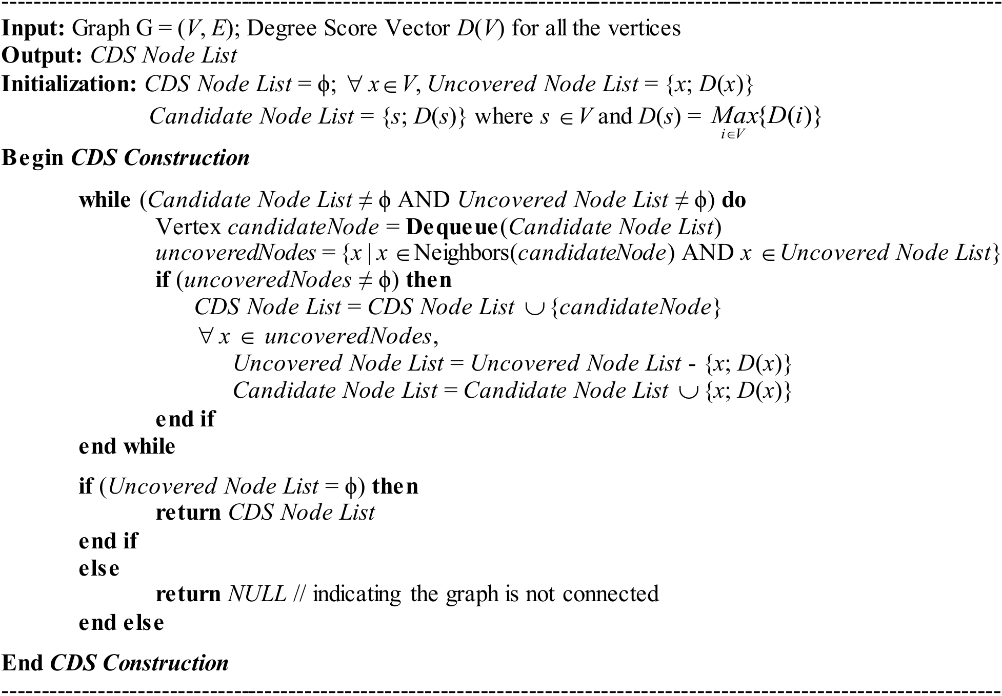
The time complexity for the CDS construction heuristic is O(VlogV + ElogV), where V and E are respectively the number of vertices and edges in the network graph; O(logV) is the time complexity for a dequeue operation in a priority queue (Candidate Node List) maintained as a Max-Heap [8] as well as the time complexity to include a vertex in the Candidate Node List by visiting the neighbors of the vertex that is added to the CDS Node List. We could run the while loop at most V times, once for each vertex, and across all such iterations, the entire set of edges are traversed and the end vertices of the edges are considered for inclusion to the Candidate Node List. Hence, the overall time complexity of the generic heuristic to construct a degree-based CDS is O((V+E) logV).
2.2 Example to Construct Degree-based CDS
In this section, we show the execution of the degree heuristic on a sample network graph. For each vertex in Figure 2, the ID is indicated inside the circle and the degree of the vertex is indicated outside the circle. The last graph in each of these figures is a CDS graph comprising of only edges between two CDS nodes (indicated as solid lines) and edges between a non-CDS node and a CDS node (indicated as dotted lines).
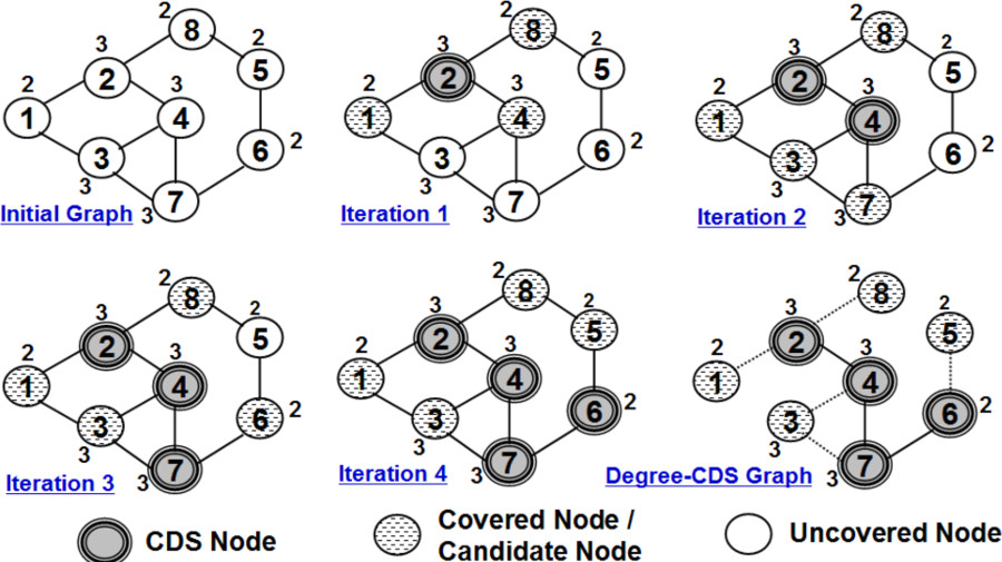
Figure 2 illustrates the execution of the heuristic to determine degree-based CDS: in iteration 3, even though vertices 3 and 7 have the same larger degree (3), vertex 3 is not considered for inclusion to the CDS because all of its three neighbors are already covered (i.e., none of the neighbors of vertex 3 are in the Uncovered Node List); on the other hand vertex 7 has one uncovered neighbor and is hence included to the CDS Node List. The sequence of vertices included in the Degree-based CDS are 2, 4, 7 and 6. One significant observation could be made in the toy example shown in Figure 2: Vertex 3 with a relatively higher degree (3) is connected to two high-degree vertices (vertices 2 and 7), but does not contribute much in terms of covering nodes that are yet in the Uncovered Nodes List once vertices 2 and 7 get into the CDS Node List. Thus, vertex 3 is a highly enclosed vertex that is not exposed much to vertices outside its own community. On the other hand, even if vertex 2 gets into the CDS Node List, vertex 7 could also get into the CDS Node List, because they are connected to two different vertices/communities (vertices 8 and 6) that only either of them could cover, but not both.
2.3 Algorithm to Validate the Existence of a CDS
We now present the algorithm that we use to validate the existence of a CDS at any time instant. This algorithm would be very useful in discrete-event simulations when we tend to use a CDS that existed at an earlier time instant (say, t-1) at a later time instant (t). That is, given a CDS Node List that was connected (i.e., the CDS nodes are reachable from one another directly or through one or more intermediate CDS nodes) and covered the non-CDS nodes in the network graph at time instant t-1, we want to validate whether the same holds true at time instant t. We do so by first constructing a CDS graph based on the CDS Node List at time instant t. All the vertices in the network are part of the CDS graph and the edges in the CDS graph are those that exist between any two CDS nodes as well as between a CDS node and a non-CDS node at time instant t. We check if the CDS Node List is connected at time instant t by running the Breadth First Search (BFS) 8 algorithm, starting from an arbitrarily chosen CDS node and see if every other CDS node could be reached as part of the BFS traversal only on the CDS-CDS edges. If all the CDS nodes could be visited, the CDS Node List is considered to be connected. We then check whether every non-CDS node has an edge to at least one CDS node at time t. If both the validations (connectivity of the CDS Node List and coverage of every non-CDS node by at least one CDS node) are true, then we consider the CDS to exist at time instant t.
3 Benchmarking Algorithm for Maximum Stability Connected Dominating Set
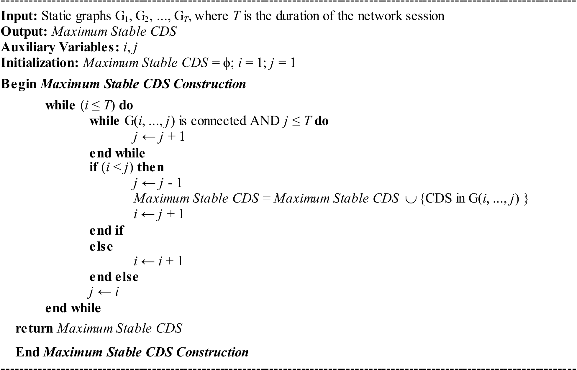
In this section, we describe a benchmarking algorithm [9] proposed to determine a sequence of longest-living connected dominating sets for MANETs such that the number of transitions is the global minimum and the average lifetime of the CDS is the maximum. We refer to the algorithm as the Maximum Stable CDS algorithm; it works on the basis of graph intersections and assumes the availability of information about topology changes for the entire duration of the network session. The algorithm introduces the notion of a mobile graph G(t, ...., t+k) = G(t)
As seen in the pseudo code for the Maximum Stable CDS algorithm (Figure 3), it does not matter what CDS construction heuristic we use to determine a CDS in each of the longest-living mobile graphs G(i, ..., j), because the CDS would not exist in the mobile graph G(i, ..., j+1) as the latter would not be a connected graph. In this research, we determine the connected dominating sets in the longest-living mobile graph G(i, ..., j) based on the degree of the vertices in the mobile graph G(i, ..., j). The average lifetime of the Maximum Stable CDS would not be affected because of this; however, the size of the Maximum Stable CDS is likely to be affected. As degree-based CDSs are likely to incur a lower CDS Node Size, it would be only appropriate to determine the connected dominating sets in each of the longest-living mobile graphs G(i, ..., j) using the degree of the vertices in the mobile graph so that the Maximum Stable CDS would incur a lower CDS Node Size and at the same time incur the maximum lifetime. The time complexity of the Maximum Stable CDS algorithm depends on the time complexity of the underlying heuristic used to determine the CDSs in each of the mobile graphs. As one can see in the pseudo code (Figure 3), there could be at most T mobile graphs (where T is the number of static graph snapshots, number of graph samples) on which a CDS heuristic needs to be run; if we use a Θ (V 2) heuristic to determine degree-based CDSs, then the overall time complexity of the Maximum Stable CDS algorithm is O(V 2 T).
3.1 Proof of Correctness
We now present an informal proof of correctness of the Maximum Stable CDS algorithm. For a more formal proof, the interested reader is referred to 9. To prove that the Maximum Stable CDS algorithm finds a sequence of long-living CDSs that incur the minimum number of transitions (say m), assume the contrary - i.e., there exists a hypothetical algorithm that determines a sequence of CDSs that undergo n transitions such that n < m. We will now explore whether this is possible. For n < m to exist, there has to be an epoch of time instants [p, ..., s] that is a superset of an epoch of time instants [q, .., r] such that p < q < r < s and that the hypothetical algorithm was able to find a CDS that existed during time instants [p, ..., s], but the Maximum Stable CDS algorithm can only find a CDS that existed during time instants [q, ..., r] and had to go a transition at time instant r + 1. This implies the Maximum Stable CDS algorithm could not find a connected mobile graph G(q, ..., r+1) and could only find a connected mobile graph G (q, ..., r). This means there existed no connected mobile graph from time instants [ q, ..., s] and hence there is no connected mobile graph from time instants [p, ..., s]. If that is the case, it would not be possible to find a CDS that exists from time instants [p, ..., s]; thus, the sequence of connected dominating sets determined by the hypothetical algorithm has to undergo at least as many transitions as those determined by the Maximum Stable CDS algorithm, which is a contradiction to our initial assumption that n < m. Hence, the number of transitions (m) incurred by the sequence of long-living CDSs determined by the Maximum Stable CDS algorithm serves as a lower bound for the number of transitions (n) incurred by any other algorithm/heuristic to determine a sequence of CDSs.
3.2 Example
Figure 4 presents an example to illustrate the execution of the Maximum Stable CDS algorithm on a sequence of five static graphs G1, ..., G5 and a comparison of the number of transitions (changes from one CDS to another) and CDS Node Size incurred for Maximum Stable CDS vis-a-vis a degree-based CDS on the same sequence of static graphs. We see that there exists a connected mobile graph G(1, 2, 3) and a connected mobile graph G(4, 5). Hence, it would suffice to use one CDS determined on the mobile graph G(1, 2, 3) and another CDS determined on the mobile graph G(4, 5) - resulting in only one CDS transition across the five static graphs. On the other hand, the degree-based CDS determined on an individual static graph does not exist in the subsequent static graph. Hence, we end up determining a new degree-based CDS on each of the five static graphs - resulting in a total of four CDS transitions across the five static graphs. In Figure 4, we use a degree-based heuristic to determine a CDS on each of the two mobile graphs.
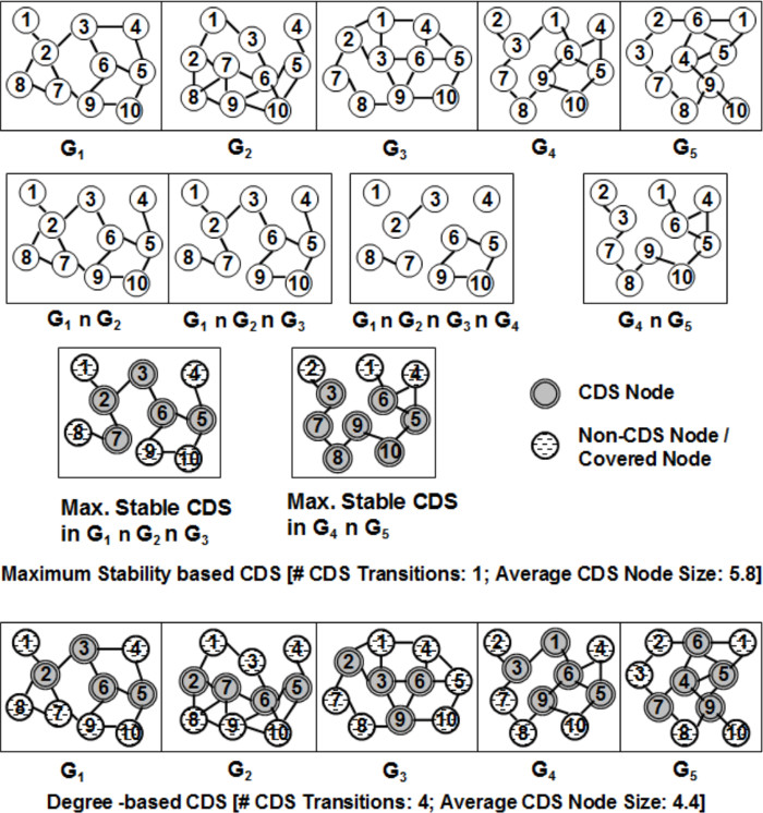
Figure 4: Example to Illustrate the Execution of the Maximum Stable CDS Benchmarking Algorithm and a Comparison of Maximum Stable CDS vs. Degree-based CDS
We do observe a tradeoff between CDS Node Size and the number of CDS transitions. The average CDS Node Size incurred for the Maximum Stable CDS is (3*5 + 2*7) / 5 = 5.8, whereas the average CDS Node Size incurred for degree-based CDS is (3*4 + 2*5) / 5 = 4.4. The mobile graphs G(1, 2, 3) and G(4, 5) have relatively fewer links than the individual static graphs. Hence, it is not possible to cover a larger number of nodes with the inclusion of few nodes in the CDS. As a result, the Maximum Stable CDS incurs a relatively larger CDS Node Size compared to that of the degree-based CDS.
4 Simulations
We conducted the simulations in a discrete-event simulator implemented in Java. We assume a network of dimensions 1000m x 1000m; the number of nodes is fixed as 100 and the transmission range of the nodes is fixed at 250m; for these values, on average, there are π*250*250*100/(1000*1000) = 20 neighbors per node. The overall connectivity of the network for the above conditions is observed to be more than 99.5%. Initially, the nodes are uniform-randomly distributed throughout the network. The number of static nodes in the network is varied with values of 0, 20, 40, 60 and 80. Since the total number of nodes in the network is 100, the above values for the number of static nodes also represent the percentage of static nodes in the network. A node designated to be static in the beginning of the simulation does not move at all for the duration of the simulation; likewise, a node designated as mobile - keeps moving for the entire simulation.
The node mobility model used is the Random Waypoint Model 10, wherein the maximum velocity of each mobile node is vmax and it is varied with values of 5 m/s (low mobility), 25 m/s (moderate mobility) and 50 m/s (high mobility). According to the Random Waypoint Model, each mobile node starts from its initial location and chooses to move to an arbitrary location (located within the network boundaries) with a velocity that is uniform-randomly selected from the range [0, ..., vmax ]; after moving to the chosen location, the node chooses another arbitrary location (within the network) and moves to the chosen location with a new velocity that is uniform-randomly chosen from the range [0, ..., vmax ]. In other words, a node moves in a straight line from one location to another chosen location with a particular velocity and after reaching the targeted location, the node chooses another target location to move with a velocity that could be different from the one used before. A mobile node moves like this for the duration of the simulation session and generates a mobility profile for a particular combination of values for the number of static nodes and maximum node velocity. The collection of the mobility profiles of all the nodes is stored in a mobility profile file and is feed in to the heuristic/algorithm for determining a degree-based CDS and the Maximum Stable CDS. We generate 100 such mobility profile files for each of the combinations of the values for the number of static nodes (0, 20, 40, 60 and 80) and the maximum node velocity (5 m/s, 25 m/s and 50 m/s). The decision of whether a node will be static or mobile is made prior to creating each of the mobility profile files.
We run the simulations for each mobility profile file and average the results observed for the CDS Lifetime and CDS Node Size for the degree-based CDS as well as the Maximum Stable CDS. We start the simulations at time 0 sec (based on the initial distribution of the nodes in a particular mobility profile file) and run the simulations for a period of 1000 seconds, sampling the network for every 0.25 seconds of the simulation. We take a snapshot of the network at each of these sampling time instants (referred to as the static graphs). We use the following approach to run the simulations for the degree-CDS: Whenever a CDS is needed at a particular time instant t, we determine the degree scores of the nodes based on the static graph snapshot of the network at time instant t and feed in these scores to the CDS construction heuristic (described in Section 2.1). The CDS determined at time instant t is used for the subsequent sampling time instants as long as it exists (validated using the algorithm presented in Section 2.3). When the currently known CDS is observed to no longer exist at a particular time instant, we repeat the above procedure. We continue like this for the duration of the simulation and measure the lifetime and node size for the sequence of degree-based connected dominating sets used for the particular mobility profile file. We average the results for these two metrics (Figures 5, 6, 7) observed for all the mobility profile files generated for a particular combination of values for the number of static nodes and vmax . In the case of the Maximum Stable CDS algorithm, for a particular simulation run under a mobility profile file, we determine a sequence of connected mobile graphs for the duration of the simulation session and run the degree-based CDS construction heuristic to determine a sequence of connected dominating sets. We repeat this procedure for all the mobility profile files generated and determine the average of the lifetime and node size for the sequence of Maximum Stable CDSs for the particular combination of values of the number of static nodes and vmax .
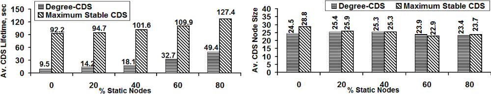
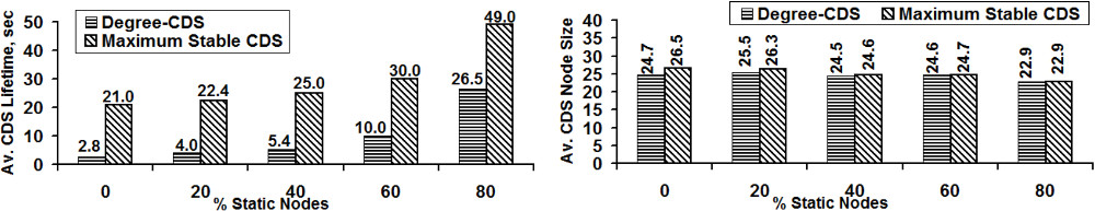
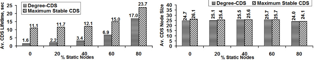
As expected, the Maximum Stable CDS incurred a larger CDS lifetime compared to that of the degree-based CDS. However, for any given level of node mobility (vmax ), the difference in the CDS lifetimes between the Maximum Stable CDS and degree-based CDS significantly decreases with increase in the percentage of static nodes in the network. For vmax = 5 m/s, the ratio of the lifetime of the Maximum Stable CDS to that of the degree-based CDS decreases from a factor of about 10 to 2.5 as we increase the percentage of static nodes from 0 to 80. As the value of vmax increases, the reduction in the difference is even more prominent. For vmax = 25 m/s, the ratio of the lifetime of the Maximum Stable CDS to that of the degree-based CDS decreases from a factor of about 7.5 to 1.8; and for vmax = 50 m/s, the ratio of the lifetimes decreases from a factor of about 7 to 1.4. Thus, the lifetime of degree-based CDS becomes very comparable to that of the Maximum Stable CDS when 80% of the nodes in the network are static and only 20% are mobile. In general, when more than half of the nodes in the network are static, the lifetime of the degree-based CDS starts to swiftly approach the lifetime of the Maximum Stable CDS. Thus, as predicted in our hypothesis, the presence of static nodes in the network has a very positive effect on the stability of the degree-based CDSs, but only a marginal effect on the lifetime of the Maximum Stable CDS.
The lifetime of the degree-based CDSs increases by a factor of 5 to 13 as we increase the percentage of static nodes from 0 to 80; the increase is substantial with increase in the level of node mobility. At vmax = 5 m/s, the increase in the lifetime of the degree-based CDSs is by a factor of 5 as we increase the percentage of static nodes from 0 to 80; however at vmax = 25 m/s and 50 m/s, the lifetime of the degree-based CDSs increases by a factor of 10 to 13. At the same time, the node size for the degree-based CDSs remains slightly high when the percentage of static nodes is low (0, 20 or 40) and then again decreases by a factor of at most 20% when the percentage of static nodes increases to 60 and 80. Thus, we observe the presence of static nodes in the network to significantly increase the lifetime and even marginally reduce the node size for the degree-based CDSs, thereby reducing the stability-tradeoff appreciably. We observe the lifetime of the Maximum Stable CDS to increase at most by a factor of 2.3 with increase in the percentage of static nodes. Like it was observed for the degree-based CDSs, the increase is only about 40% when vmax = 5 m/s and is higher for vmax = 25 m/s and 50 m/s; similarly, the node size for the Maximum Stable CDSs decreases by about 20% with increase in the percentage of static nodes. We observe the node size for the Maximum Stable CDS to converge towards the node size of the degree-based CDS with increase in the percentage of the static nodes.
5 Related Work
MANET simulation studies have typically used the Random Waypoint model as the mobility model. As per this mobility model, a mobile node moving in a particular direction could pause for a certain time after reaching a targeted location and then continue to move. The pause time is one of the parameters of the Random Waypoint mobility model. The influence of static nodes on the performance of a communication protocol has been so far evaluated only on the basis of this pause time. Also, such studies have been typically conducted to analyze the performance of unicast routing protocols (e.g., 11)) and multicast routing protocols (e.g., 12)) for MANETs. Even in such works, the focus had been on the impact of pause time on metrics such as delay, throughput, energy consumption, etc, but not explicitly on the lifetime of the communication topologies like paths and trees. To the best of our knowledge, we have not come across any studies that consider the influence of static nodes of any form (including pause time) on the performance of network-wide communication topologies, like that of connected dominating sets for MANETs. In this paper, we chose to designate certain nodes as static throughout the simulation and let the other nodes to move (rather than letting all mobile nodes to move and pause alternately). We wanted to see if the presence of static nodes (nodes that do not move at all) could improve the overall stability of connected dominating sets (as it is seen in the simulations) so that we could henceforth come up with a network design strategy wherein even though certain nodes in a network are bound to be mobile all the time, one may deploy certain percentage of static nodes that could significantly increase the stability of network-wide communication topologies such as connected dominating sets.
6 Conclusions
The simulation results confirm our hypothesis: We observe that for a given level of node mobility, the lifetime of the Maximum Stable CDS does not increase substantially with increase in the percentage of static nodes; on the other hand, the lifetime of the degree-based CDS increases significantly (and approaches the lifetime of the Maximum Stable CDS) with increase in the percentage of static nodes. As we increase vmax from 5 m/s to 50 m/s, the average lifetime incurred for the Maximum Stable CDS increases by a factor of 1.4-2.3 as we increase the percentage of static nodes from 0 to 80. This could be attributed to the fact that the mobility of certain percentage of nodes is sufficient to disrupt the connectivity of the mobile graphs spanning over several time instants. On the other hand, as we increase vmax from 5 m/s to 50 m/s, the lifetime of the degree-based CDS increases substantially (by factors as large as 13) with increase in the percentage of the static nodes from 0 to 80. Thus, even if a certain fraction of nodes move faster, the presence of a significant fraction of static nodes helps to boost the lifetime of the degree-based CDS. In this paper, the degree-based CDS heuristic did not take into account the presence of static nodes while considering nodes for inclusion in the CDS. With the results observed in this paper, we anticipate that if the heuristic is adapted to take into account both the node velocity (or some form of node mobility) and node degree while forming a CDS, the stability of such CDSs could be significantly higher than that incurred with CDSs determined using a degree-based heuristic without any appreciable increase in the CDS node size. We thus anticipate the results of this paper to open new avenues of research for improving the stability of degree-based heuristics for MANETs.

