


 text new page (beta)
 English (pdf)
 Article in xml format
 Article references
 Send this article by e-mail
 Cited by SciELO
  Similars in
SciELO
Similars in
SciELO 
 Permalink
1 Introduction
Guillain-Barré Syndrome (GBS) is an autoimmune neuropathy of fast evolution and potentially fatal. GBS has an incidence of 1.3 to 2 per 100,000 people and a mortality rate from five to fifteen percent. The exact cause of GBS is unknown; however, it is frequently preceded either by a respiratory or a gastrointestinal infection. The diagnosis of GBS includes clinical, serological and electrophysiological criteria (nerve conduction or Electrodiagnostic test) 1. The severity of GBS varies among subtypes, which can be mainly Acute Inflammatory Demyelinating Polyneuropathy (AIDP), Acute Motor Axonal Neuropathy (AMAN), Acute Motor Sensory Axonal Neuropathy (AMSAN) and Miller-Fisher Syndrome 2. Electrodiagnostic criteria for distinguishing AIDP, AMAN and AMSAN are well established in the literature 3, while the Miller-Fisher subtype is characterized by the clinical triad: ophthalmoplegia, ataxia and areflexia 2. In Mexico, axonal subtypes are prevalent 4, 5.
A better understanding of the differences in the GBS subtypes is critical for the implementation of appropriate treatments for total recovery and, in certain cases for the survival of patients. Hospitalization time and the cost of treatments vary according to the severity of the specific subtype. Finding a minimum feature subset to accurately identify GBS subtypes could lead to a simplified and cheaper process of diagnosis and treatment of the GBS case. The ultimate goal of a physician is to get patients to a full recovery. This can be more effectively achieved when an early diagnosis of the case is performed using a minimum number of medical features.
Cluster analysis or clustering is a machine learning technique that allows to group objects into clusters. Objects in the same cluster are similar and dissimilar from objects in other clusters. Cluster analysis has applications in many disciplines 6, 7, 8. Particularly, cluster analysis has been used in medicine to identify disease subtypes 9, 10, 11, among other applications.
In this work we use a real dataset consisting of 156 features and 129 cases of GBS patients, these are 20 AIDP cases, 37 AMAN, 59 AMSAN and 13 Miller-Fisher cases. The dataset contains clinical, serological and nerve conduction test data.
This work constitutes an initial exploratory analysis of our dataset using machine learning techniques. We started with a clustering technique as this method is useful to study the internal structure of data to disclose the existence of groups of homogeneous data. We know in advance of the existence of four GBS subtypes or classes in our dataset. It is our interest to investigate the capability of computational algorithms such as clustering techniques to identify these four real groups using a minimum number of features. Machine learning techniques has been found in the literature to predict the prognoses of this syndrome 12,13 as well as to find predictors of respiratory failure and necessity of mechanical ventilation in GBS patients 14, 15, 16. Nevertheless, no previous studies on cluster analysis of GBS data using machine learning techniques were found in the literature.
Usually in cluster analysis there is no prior information as a guide to find the exact number of clusters and therefore different partitions with different number of clusters are explored. The ultimate goal is to select the highest quality partition, based on an internal or external metric. In this work, we perform a cluster analysis in a real GBS dataset to identify relevant features that allow to build four clusters, each corresponding to a GBS subtype. The quality of the clusters is measured with an external metric called purity. Purity is an external clustering validation metric that evaluates the quality of a clustering based on the grouping of objects into clusters and comparing this grouping with the ground truth. The high purity is reached when clusters contain the largest number of elements of the same type and the fewest number of elements of a different type. Although there are several clustering validation metrics, both internal and external 17, we selected purity since our interest was to find "pure" groups and to take advantage of the available prior knowledge of the true labels. The use of a prior knowledge to evaluate a clustering process is also known as supervised or semi-supervised clustering, some examples can be found in 18, 19, 20, 21.
Our approach consists of a combination of Quenching Simulated Annealing (QSA) and Partitions Around Medoids (PAM), which we named as QSA-PAM method. PAM algorithm is used to perform the clustering process and is thoroughly described in section 2.2.1. Simulated Annealing (SA) is a general purpose randomized metaheuristic that finds good approximations to the optimal solution for large combinatorial problems. The SA algorithm was proposed by Kirkpatrick et al. 22 and Cerny 23 and is an extension of the Metropolis algorithm 24. This method takes its name from the metallurgy field where there is a process in which a piece of metal is initially heated to high temperatures and then gradually cooled to change the configuration of atoms in order to reach a thermal equilibrium. In a similar fashion, the computational version of this process uses a cooling scheme to control the pace and duration of the search for the best solution. At a high temperature, SA widely explores the solution space and accepts worse solutions than a current one with a high probability, which let SA avoids getting stuck in local minima. As the temperature goes down, the searching process becomes stricter and the probability of accepting a bad solution becomes increasingly low.
QSA is a version of SA consisting of two phases: Quenching and Annealing 25. In the Quenching phase the temperature is quickly decreased, using an exponential function, until a quasi-thermal equilibrium is reached. This phase is applied at a very extremely high temperature and its purpose is to broadly explore the feature space. The Annealing phase comes in after Quenching phase completes, where the temperature is gradually reduced. This paper is organized as follows. In section 2 we present a description of the dataset, the functioning of PAM and QSA methods, as well as the metrics used in the study and finally, we explain the QSA-PAM method. In section 3 we show how the QSA parameters were determined and also we give experimental results of QSA-PAM method. Section 4 discusses the results of the study. In section 5 we summarize conclusions of the study and also we suggest some future works.
2 Materials and methods
2.1 Data
Records of 129 patients attended at Instituto Nacional de Neurología y Neurocirugía in Mexico City were used for experiments in this work. Data were collected from 1993 through 2002. There are 20 AIDP cases, 37 AMAN, 59 AMSAN and 13 Miller-Fisher cases. The identification of subtypes was made by a group of neurophysiologists based on the clinical and electrophysiological criteria established in the literature 1, 2. In this study, each subtype represents a class. Therefore, there are four classes in the dataset. This dataset is not yet publicly available and this is the first time it is used in an experimental study. No public dataset was found to be used as a benchmark.
Originally, the dataset consisted of 365 attributes corresponding to epidemiological data, clinical data, results from two nerve conduction (electrodiagnostic) tests, and results from two Cerebrospinal Fluid (CSF) analyses. The second nerve conduction test was conducted in 22 patients and the second CSF analysis was conducted in 47 patients only. Therefore, data from these two tests were excluded from the dataset.
The diagnostic criteria for GBS are established in the literature 1, 2. These formal criteria were considered to determine which variables from the original dataset could be important in the characterization of the four subtypes of GBS. We made a pre-selection of variables based on these criteria. After pre-selection, the dataset was left with 156 variables: 121 variables from the nerve conduction test, 4 variables from the CSF analysis and 31 clinical variables. As for the type of attributes, these are 28 categorical and 128 numeric attributes. The situation of dealing with mixed data types was solved using Gower's similarity coefficient, as explained later in section 2.4.
2.2 Methods
2.2.1 Partitions Around Medoids (PAM)
As stated before, the dataset used in this work combines categorical and numeric data. PAM is a clustering algorithm capable of handling such situations. It receives a distance matrix between instances as input. The distance matrix was computed using Gower's coefficient, described in section 2.4.
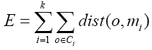
PAM, introduced by Kaufman and Rousseeuw 26, aims to group data around the most central item of each group, known as medoid, which has the minimum sum of dissimilarities with respect to all data points. PAM forms clusters that minimize the total cost E of the configuration, that is, the sum of the distances of each data point with respect to the medoids. E is formally defined as:
 (1)
(1)
where k is the number of clusters, o ϵ Ci is the set of objects in the cluster Ci, and dist(o, mi) is the distance between an object o and a medoid mi.
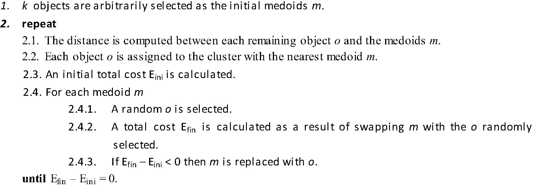
PAM works as shown in Algorithm 1 27:
2.2.2 Clustering validation measure
The dataset used in this work provides the ground truth. We know there are four classes in the dataset. The goal of this study was to find a minimum set of features that as purely as possible identify four clusters, each corresponding to one class. To achieve this goal we selected purity as the metric to evaluate the quality of the clustering process.
Purity validates the quality of a clustering process based on the location of data in each cluster with respect to the true classes. The more objects in each resultant cluster belong to the true class, the higher the purity. Formally 28:
 (2)
(2)
where N is the number of labeled samples, Ω = {W1, W2, ..., Wk} is the set of clusters found by the clustering algorithm, C = {C1, C2, ..., Cj} is the set of classes of the objects, K is the number of clusters, J is the number of classes, wk
is the set of objects in cluster k, cj
is the set of objects in class
2.2.3 Gower's similarity coefficient
Distance metrics are used in clustering tasks to compute the distance between objects. The distance computed is used by clustering algorithms to determine how similar or dissimilar the objects are. Based on it, a clustering algorithm can determine which cluster the objects could be thrown in. There are many distance metrics. Some of them deal with numeric data, such as Euclidean, Manhattan and Minkowski 27. To deal with binary data, the Jaccard coefficent and Hamming are often used 27. For categorical data, some distance metrics are Overlap, Goodall and Gambaryan 29.
In this work we used for experimentation a dataset that contains mixed data, that is, both categorical and numeric data. To deal with this context we selected the Gower's coefficient. It is a robust and widely used distance metric for mixed data. We used this coefficient to obtain a matrix of distances between instances as required by PAM. It was introduced by Gower in 1971 30. Gower's coefficient is defined as follows 31:
 (3)
(3)
 (4)
(4)
where p1 is the number of quantitative variables, p2 is the number of binary variables, p3 is the number of qualitative variables, a is the number of coincidences for qualitative variables, a is the number of coincidences in 1 (feature presence) for binary variables, d is the number of coincidences in 0 (feature absence) for binary variables, and Gh is the range of the h-th quantitative variable.
Gower's coefficient is within the range 0 - 1. A value near to 1 indicates strong similarities between items and a value near to 0 indicates weak similarity.
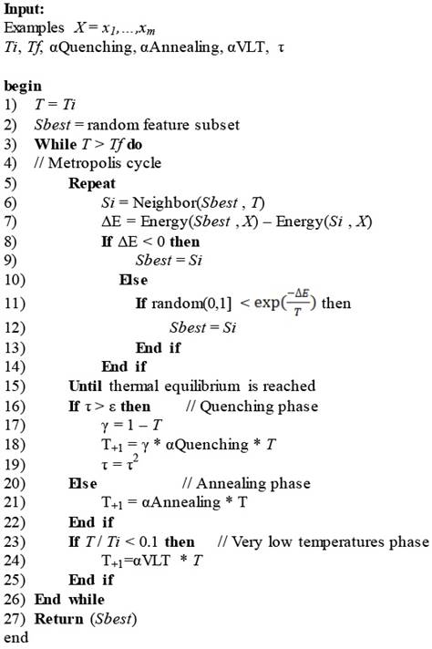
2.2.4 Quenching Simulated Annealing (QSA)
In this work we aim to find a minimum feature subset for identifying four GBS subtypes from a 156-feature real dataset. This represents a combinatorial problem and to find a good approximation of the best solution the QSA metaheuristic was selected. QSA, shown in Algorithm 2, is a version of the SA algorithm which has two phases: Quenching and Annealing. Quenching phase is applied at a very high temperature which is rapidly reduced using an exponential function until a quasi-thermal equilibrium is reached. Quenching phase has shown to allow the exploration of a wider portion of the solution space than previous SA approaches did 32. In Annealing phase the temperature is gradually reduced and therefore the exploration is performed at a slower pace, and so the solution space is scrutinized aiming to find the best solution. Figure 1 shows the temperature behavior in both Quenching and Annealing phases.
The classical SA algorithm receives as input a set X of m examples with n features. Classical SA requires a triplet composed of an Annealing schedule, an Energy function and a neighbour function. The Annealing schedule is defined by the initial temperature Ti, the final temperature Tf and the Annealing constant αAnnealing. These values control the pace and duration of the search. The Energy function evaluates the quality of a solution. The goal of SA is to optimize this function. In this particular problem we used the purity measure as the Energy Function. The neighbour function receives both the current solution and temperature as input and returns a new candidate solution that is nearby to the current solution, in terms of the variation of features between both solutions. For high values of T a broader search in the dataset is performed to generate Si. For low values of T the search becomes almost local.
QSA also behaves different with respect to the energy function in Quenching and Annealing phases (Figure 2). In Quenching phase, the energy function undergoes high fluctuations as QSA is still exploring the search space. As Annealing phase advances, the fluctuations in the energy function decrease as in this phase QSA is now looking for the best solution. At the end of Annealing, the energy function in fact remains stable.

QSA uses two extra parameters: a Quenching constant α Quenching and τ. These parameters work together to reduce the temperature at a rapid pace until τ converges to ε. In addition, this particular implementation uses a cooling constant αVLT at very low temperatures, which enables the search space to be meticulously traversed, which corresponds to performing a local search.
QSA, shown in Algorithm 2, begins initializing the value of T (line 1). A random feature subset is taken as an initial best solution Sbest (line 2). In this implementation the initial size of Sbest (between 2 and 156 variables inclusive) and their elements are randomly selected using the Mersenne-Twister pseudo random number generator. An external cycle is performed for controlling temperature variations until Tf (line 3) is reached. The Metropolis cycle (nested loop of lines 5-15) is performed until "thermal equilibrium" is reached. In this cycle, a neighbor solution Si is generated using Sbest and the value of T (line 6). The Neighbor function draws a new state Si based on the precious state Sbest where a number of features in Sbest is replaced with new features randomly taken from the original dataset depending on the current temperature T. For high values of T, a maximum of 80% of the features are replaced. For low values of T, a maximum of 20% of them are replaced. The difference in energy ∆E between Sbest and Si is calculated (line 7) If ΔE < 0, that is Si is a better solution than Sbest (line 8), then Si becomes the best solution (line 9). If ΔE > = 0, it means Si is a worse solution than Sbest, then the best solution Sbest is replaced with Si only if a random number generated in the range [0,1) is less than
2.2.5 Description of QSA-PAM method
The method we introduced in this work is a combination of two methods: Quenching Simulated Annealing (QSA) and Partitions Around Medoids (PAM), named QSA-PAM method (Figure 3). This is a novel method in machine learning implemented to search a large search space for a feature subset that leads to a good solution for a clustering problem. In our work, QSA-PAM was used to solve the problem of identifying four GBS subtypes - AIDP, AMAN, AMSAN and Miller-Fisher - with the highest purity possible. The method is described below.
QSA-PAM receives a dataset with n features as input. In this particular implementation n = 156. The class attribute was excluded as required in a clustering problem. We used it as the ground truth to compute the purity of the clusters obtained with PAM. For all experiments, the number of clusters requested to PAM algorithm was k = 4, as there are four GBS subtypes present in the dataset.
The method works as follows (see Figure 3): a cycle from i = 2 to n is performed. For each value of i, QSA finds the best feature subset containing up to i features that identify four clusters with the highest purity (e.g. for i equals 25 the best feature subset could be of size 18). At each iteration, different feature subsets (size varying from 2 to i) from the entire dataset are chosen by QSA algorithm. New datasets are created with each of these feature subsets. A distance matrix between instances from these new datasets is computed using Gower's similarity coefficient which is used as input to PAM to build four clusters. The calculation of the distance matrix requires at least 2 attributes, and this is the reason for using a minimum value of i = 2 in the main loop (For i = 2 to n variables). Finally, the purity of the clusters is computed as it is used as the energy function in QSA. QSA finds the feature subset that optimizes the energy function for each value of i. The aim of having QSA selecting the best features for each value of i is to look into the number of times such variables get selected, this would give us insight on their relevance. That is, the more times a variable is selected the more relevant it is.
As a result of the method we obtained a list of feature subsets that build four clusters with the highest purity possible for each value of i, each corresponding to a GBS subtype. In other words, the list contains the best 2-feature subset, the best 3-feature subset, and so on up to the best 156-feature subset.
In this study we perform a number of runs of QSA-PAM. For each run, we set a different seed. These seeds were generated using Mersenne-Twister pseudo random number generator 33. Using a different seed for each run of QSA-PAM allows for QSA part of the method to generate different combinations of feature subsets from the search space to choose from.
3 Results
3.1 Determination of QSA parameters
For tuning the proposed algorithm, we started determining the initial and final temperatures Ti and Tf respectively used by QSA part of our method. These temperatures are computed as follows 25:
 (5)
(5)
 (6)
(6)
Where ΔZmax and ΔZmin are the maximal and the minimal deterioration respectively, both of the energy function. Deterioration refers to changes in the Energy function, that is, the changes in purity at an extremely high temperature and extremely low temperatures for ΔZmax and ΔZmin respectively.
P(ΔZmax) and P(ΔZmin) are the probabilities of accepting a new solution with ΔZmax and ΔZmin respectively. The probability of accepting a new solution is close to 1 at extremely high temperatures and close to 0 at extremely low temperatures 25.
To determine ΔZmax and ΔZmin, 30 runs of QSA-PAM were performed using random samples from the 156-feature dataset. Different arbitrary temperature values, in the range [7.674419x10⁶, 1x10⁻⁵] were used. An average value of 0.1372 was obtained for ΔZmax and 0.0088 for ΔZmin. Using both equations in 5 and 6 led us to temperatures of 1.376999x10⁶ for Ti and 7x10⁻⁴ for Tf. We used these values as approximations to the final temperatures. To verify the quality of these values, three different combinations of Ti and Tf were used and compared in 30 runs of QSA-PAM: the values obtained with equations 5 and 6 (Ti = 1.376999x10⁶ and Tf = 7x10⁻⁴), an arbitrary higher temperature combination (Ti = 1.5x10⁶ and Tf = 1x10⁻³) and other arbitrary lower temperature combination (Ti = 1x10⁶ and Tf = 1x10⁻⁵). The purity values obtained across 30 runs were averaged for every temperature combination. Results are shown in Table 1.
Table 1 Average purity over 30 runs of QSA-PAM using three different temperature configurations.
| Ti | Tf | Average best solution (purity) after 30 runs of QSA-PAM |
|---|---|---|
| 1.5x10⁶ | 1x10⁻³ | 0.7509 |
| 1.376999x10⁶ | 7x10⁻⁴ | 0.7564 |
| 1x10⁶ | 1x10⁻⁵ | 0.7881 |
Values of α and τ were assigned according to values typically used in literature 25, 34, 35. Values for QSA parameters are shown in Table 2.
3.2 Experimentation
3.2.1 Finding clusters using the 156-feature dataset
The aim of the initial experiments was to analyse the behaviour of clusters using the whole 156-feature dataset. In order to achieve our goal, QSA-PAM was run 30 times using the 156-feature dataset, each run with a different seed. In each run, a list of the best feature subset for i equals 2 to 156 was obtained. Then, the purity of clusters obtained using each of the feature subsets was calculated. Finally, the average purity of clusters over 30 runs for each value of i was computed. The results are shown in Figure 4. The chart shows an initial ascending behaviour, a peak is reached approximately at I equals 30 and then the chart begins to slowly descend. The average purity values ranged in [0.75, 0.80]. We want to highlight that two feature subsets in the feature space over 30 runs reached a maximum purity of 0.8527. Also, by looking at Figure 4 we identified the need of determining a proper number of features to be used to create clusters of high purity.

3.2.2 Analysis of the size of the feature subsets selected by QSA-PAM
With the aim of determining the proper number of features selected by QSA-PAM, we further analyzed the size of the resultant feature subsets. QSA-PAM selects the best feature subset that maximizes the purity of four clusters for each value of i ranging in [2,156]. The size of these feature subsets would not necessarily match the value of i. That is, for i equals 38 the size of the best feature subset could be 12 in one run, and 23 in another run. We were interested in investigating the median of the best feature subsets for each value of i over 30 runs. To achieve this, we counted the number of features selected by QSA-PAM in each run for every value of i and then we calculated its median. The results are shown in Figure 5. Overall, the size median of the feature subsets selected by QSA-PAM was less than 50, even in cases where a number greater than 100 was requested.
3.2.3 Analysis of frequencies of features selected by QSA-PAM
We also investigated the total frequency of selection by QSA-PAM for each feature in the dataset along the 30 runs, as shown in Figure 6. A ranking for all the 156 features was created based on these frequencies. That is, the feature on top of this ranking is the most frequently selected features. The highest frequency possible for any feature over 30 runs was 4650, that is 155 x 30 (155 total features, 30 runs). The highest frequency obtained for a feature was 2612. Five features stood out of all the 156 features reaching a frequency greater than 2000. These features were 14, 142, 13, 15 and 138 as shown in the chart. We considered to use for further experiments only features with a frequency over 1000. This number of features counted to fifty. Coincidentally, fifty was the threshold derived from the analysis described in section 3.2.2.
3.2.4 Quality of clusters formed using feature subsets based on the ranking of frequencies
Based on the ranking of features according to frequencies for all 156 features, we created new datasets using the best 2 features, the best 3 features, and so on, up to 156 features. For each of these datasets, a distance matrix was computed using Gower's similarity coefficient. Each matrix was used as input for PAM to build four clusters. Finally, the purity of clusters was computed. The results of this experiment are shown in Figure 7. The highest purity obtained with these clusters was 0.81. This showed that not necessarily a sequential grouping of features based on the ranking of features would lead us to the desired purity of 1. Two other facts observed is that a low purity of 0.7054 is reached with few features (< = 15) which is similar to that obtained (0.6976) with a large number of features (> = 125).
3.2.5 Finding clusters using the 50 most frequently selected features
We were interested in searching for a feature subset that improved the highest purity obtained (0.8527) when QSA-PAM was ran using all the 156 features. To achieve this, we created a dataset using the 50 most frequently selected features. We performed a second experiment of 30 runs of QSA-PAM, for i ranging in [2, 50]. Again, the purity of clusters obtained using each feature subset was calculated. Then, we calculated the average purity for each value of i. The results are shown in Figure 8. Again, we can observe that with a few features (< = 10) the lowest average purity is obtained. This chart shows an initial ascending behaviour until i equals 10 approximately and then it stabilizes at approximately a value of purity equals 0.85 and it remains stable until the end.
3.2.6 Our best 16-feature subset
In the second experiment of 30 runs, described in section 3.2.5, we found a feature subset that built four clusters with a purity of 0.8992. This subset contains 16 features: four clinical features and 12 features from the nerve conduction test. These features are listed in Table 3. We will further investigate this feature subset to create a predictive model.
Table 3 List of features that built 4 clusters with a purity of 0.8992.
| Feature label in the dataset | Feature name and meaning |
|---|---|
| V22 | Simmetry (Simmetry in weakness) |
| V29 | Extraocular muscles involvement (Muscles that move the eyes and represent cranial nerves) |
| V30 | Ptosis (Drooping eyelid) |
| V31 | Cerebellar involvement (Affectation of the cerebellum) |
| V63 | Amplitude of left median motor nerve |
| V106 | Area under the curve of left ulnar motor nerve |
| V120 | Area under the curve of right ulnar motor nerve |
| V130 | Amplitude of left tibial motor nerve |
| V141 | Amplitude of right tibial motor nerve |
| V161 | Area under the curve of right peroneal motor nerve |
| V172 | Amplitude of left median sensory nerve |
| V177 | Amplitude of right median sensory nerve |
| V178 | Area under the curve of right median sensory nerve |
| V186 | Latency of right ulnar sensory nerve |
| V187 | Amplitude of right ulnar sensory nerve |
| V198 | Area under the curve of right sural sensory nerve |
3.2.7 Statistical analysis
We were interested in finding a region in the chart of Figure 8 where QSA-PAM could have achieved the highest average purity values. That is, we looked at diverse ranges of variables requested to QSA-PAM aiming to find a group of four clusters with the highest quality. We divided the plot into three regions (Figure 9). The first region (group A) for values of i from 3 to 18, the second region for values from 19 to 34 (Group B), and for values from 35 to 50 (Group C). The first value of i was not taken into account. These 3 groups consisted of 16 values of purity each one. We applied the non-parametric Friedman test using Holm´s correction to find statistical significant differences between purities of the three groups. The test was applied pair-wise. We took as the null hypothesis (Ho) = purity levels between two regions are the same, and as the alternative hypothesis (Ha) = purity levels between two regions are different. The results are shown in Table 4.

Table 4 Friedman-Holm test for regions A, B, and C.
| Regions compared | p Value | Ho |
|---|---|---|
| A - B | 0.317 | Accepted |
| B - C | 0.000 | Rejected |
| A - C | 1.000 | Accepted |
According to the results shown in Table 4, we found statistical significant differences between purities achieved in regions B and C as shown in Figure 9. A more extensive search in these regions could lead to a better result. That is, requesting a number of variables to QSA-PAM between 19 and 34, or between 35 and 50.
3.2.8 Temperature and energy behaviour in QSA
We show in this section the temperature and energy behaviour of QSA part of the QSA-PAM method for a single arbitrary value of i, that is for i = 50. For this value of i, the number of runs was 1002. Figure 10 shows the temperature behavior of QSA in both Quenching and Annealing phase. The quenching phase showed a rapid exponential decrease in temperature as described in the QSA section (2.2.4.). In the annealing phase, the temperature decreases slowly, as QSA searches locally in the dataset.
Figure 11 shows the energy behaviour of QSA, the purity values in this case. Being this a maximization problem, the energy behaves in an opposite way of that of the typical QSA problems. In the quenching phase, the energy had high fluctuations as it was expected. In this experiment, the fluctuations in energy in the quenching phase were between 0.48 and 0.75 approximately. These fluctuations continued in a number of runs of the annealing phase. From run 400 approximately, these changes in energy began to decrease to levels of purity of 0.62 to 0.72. From run 500 to the final run, there were three long phases of stability in the energy function. This stability is the result of QSA accepting best solutions than the current one with higher probabilities as the temperature reaches Tf. The final value of energy (purity) was 0.81.
4 Discussion
In this study we aimed to find a minimum feature subset to build four clusters, each corresponding to a GBS subtype, with the highest purity possible. In order to achieve our goal we introduced a combination of a metaheuristic (QSA) and a clustering algorithm (PAM), which we named QSA-PAM method.
As we explained in section 3.2.3, we created a ranking of all the 156 features based on the frequency of selection of each feature by QSA-PAM across 30 runs performed in an initial experiment. Using the 50 most frequently selected features, we created a new dataset to perform a final experiment consisting of 30 runs of QSA-PAM. We obtained a 16-feature subset able to build four clusters with a purity of 0.8992. In further studies, a more formal method could be used to decide on the number of most frequently selected features and use it as threshold instead of using 50. This could lead to obtain a feature subset that build clusters from GBS data with a higher purity.
The final feature subset identified in this study includes a combination of clinical and nerve conduction features. As to the four clinical features, they are reported in the literature as common clinical characteristics of GBS subtypes. This confirm the ability of QSA-PAM to select relevant clinical features for the identification of clusters. Concerning the electrophysiological features, further studies are required to confirm these findings. The identification of a minimum nerve conduction feature subset would be very useful to design a fast electrodiagnostic test.
On the other hand, this finding leads to the research question of the possibility of distinguishing the GBS subtypes investigated in this study with only one type of feature by itself, either clinical or nerve conduction feature. Specifically, a study to investigate the ability of clinical features to identify GBS subtypes is recommended. Wakerley et. al. 36 identified a set of clinical diagnostic features to classify GBS subtypes that could be used in the proposed research.
An important contribution of this study is a ranking of 156 features related with GBS. This ranking was created according to the frequency of selection of each feature by QSA-PAM across 30 runs. This ranking may be used in further studies.
With QSA-PAM, we found a 16-feature subset able to build four clusters present in our dataset with a purity of 0.8992. This finding, although able to be improved, shows the effectiveness of the method to find good solutions to clustering tasks involving feature selection.
5 Conclusions
We introduced a novel approach to find relevant features for building four clusters, each corresponding to a GBS subtype, with the highest purity possible. Our method consists of a combination of Quenching Simulated Annealing (QSA) and Partitions Around Medoids (PAM), named QSA-PAM method. Our study represents the first effort on applying computational methods to perform a cluster analysis to a real GBS dataset. An original 156-feature real dataset that contains clinical, serological and nerve conduction test data from GBS patients was used for experiments. Different feature subsets were randomly selected from the dataset using the QSA metaheuristic. New datasets created using the feature subsets selected were used as input to PAM algorithm to build four clusters, corresponding to a specific GBS subtype each. Finally, purity of clusters was measured. An initial experiment consisting of 30 runs of QSA-PAM was performed. The frequency of selection of each feature across the 30 runs was computed. A new dataset was created using the resultant top fifty features from the initial experiment and used as input to a final experiment of 30 runs of QSA-PAM. Finally, a 16-feature subset was identified as the most relevant.
The method here proposed was able to find a 16-feature subset that could build four clusters, each corresponding to a GBS subtype, with a purity of 0.8992. This result verifies the ability of metaheuristics to find good solutions to combinatorial problems in large search spaces. In addition, given a statistical significance difference between two groups of purities was found, a more exhaustive search using the maximum number of variables requested to the method associated with those groups may lead to higher purity values.
In the short term, we will investigate the use of filters to reduce the original dataset prior to the use of QSA-PAM and analyse the results.
The results of this work may help GBS specialists to broaden the understanding of the differences among subtypes of this disorder.

