


 nueva página del texto (beta)
 Inglés (pdf)
 Artículo en XML
 Referencias del artículo
 Enviar artículo por email
 Citado por SciELO
  Similares en
SciELO
Similares en
SciELO 
 Permalink
1 Introduction
The Master Bay Planning Problem (MBPP) is a combinatorial optimization problem in the context of maritime transportation. Specifically, MBPP consists of finding the best plan to stow a set of containers into another set of available locations of the containership. This problem is really difficult to solve due to the combinatorial nature of alternatives to allocate the containers 1.
When solving integer programs, an important issue is to develop good lower and upper bounds. Their importance lies in the fact that they aid with fathoming and testing for optimality. In integer programming (IP), important solution strategies consist on applying heuristic and relaxation for systematically tightening lower and upper bounds 2.
In this paper we propose two new lower bounds and two new upper bounds for the Master Bay Planning Problem. One of the lower bounds consists of relaxing an integer programming formulation for MBPP. The other three bounds are designed in a heuristic fashion. In order to test both the efficiency and the effectiveness of the lower and upper bounds, we conducted an experiment over three different sets of instances. The results show that some bounds (either lower or upper) are better when only considering either the computational time or the solution quality, independently.
We analyzed the combination of each lower bound with each upper bound, which results in four combinations. In particular, we measured two attributes: the well-known Gap and the computational time. The experimental results indicate that no combination is the best for both attributes, that is, one combination is the best considering the Gap and another is the best when considering the computational time. In order to consider both attributes together in a single statistic, we propose to evaluate a cost-benefit ratio for each combination. This ratio measures the compromise between quality and time. Thus, through this research, we allow other researchers to select the best bounds according to their own objectives.
This paper is organized in six sections. Section 2 describes the problem faced. Section 3 describes the new two lower bounds for MBPP. Section 4 presents our proposed upper bounds. Section 5 shows the experimental results and the computational analysis. Finally, Section 6 shows the conclusions.
2 Problem description
The Master Bay Planning Problem (MBPP) is an NP-hard combinatorial optimization problem 3 which is defined as follows 4. Let C and S be the set of n containers with different characteristics to be loaded on the ship and the set of m available locations on the containership, respectively. The goal is to assign each container to a location of the ship such that the total stowage time is minimized and all the given structural and operational constraints are satisfied. The 0/1 Linear Programming Model that resumes the problem was proposed by Ambrosino et. al. 5.
In the containership, the l-th location is addressed by the indices i, j, k which represent its bay, row and tier, respectively. We denote by I, J and K, respectively, the set of bays, rows and tiers of the ship, and by b, r and s their corresponding cardinality. The objective value is given by the sum of the times
The main constraints that must be considered for the stowage planning process for an individual port are related to the structure of the ship and focused on the size, type, weight, destination and distribution of the containers to be loaded. The description of each constraint is found below.
Size of containers. Usually, set C of containers is the union of two subsets, T and F, consisting, respectively, of 20 and 40 feet containers. Two contiguous locations of 20 feet are required to stow containers of 40 feet. Most of maritime companies number the bays for stowing 40' containers with even numbers. Such bays actually correspond to two contiguous bays numbered with odd numbers. The odd bays are used for the stowage of containers of 20 feet. Consequently, when a 40' container is located in an even bay (for instance bay 02), any 20' container cannot be located in the locations with the same row and tier corresponding to the two contiguous odd bays (e.g. bay 01 and bay 03).
Type of containers. Different types of containers, such as standard, carriageable, reefer, out of gauge and hazardous ones can usually be stowed in a containership. The location of reefer containers is defined by the ship coordinator (who has a global vision of the trip). Hazardous containers are also assigned by the harbormaster's office, which authorizes their loading. In particular, hazardous containers cannot be stowed either in the upper deck or in adjacent locations.
Weight of containers. The standard weight of an empty container ranges from 2 to 3.5 tons, while the maximum weight of a full container to be stowed in a containership ranges from 20-32 and 30-48 tons for 20' and 40' containers, respectively. The weight constraints force the weight of a stack of containers to be less than a given tolerance value. In particular, the weight of a stack of 3 containers of 20' and 40' cannot be greater than an a priori established value, say MT and MF, respectively. Moreover, the weight of a container located in a tier cannot be greater than the weight of the container located in a lower tier having the same row and bay and, as it is always required for security reasons, both 20' and 40' containers cannot be located over empty locations.
Destination of containers. A good general stowing rule suggests to load first (i.e., in the lower tiers) those containers having as destination the final stop of the ship and load last those containers that have to be unloaded first.
Distribution of containers. These constraints, also known as stability constraints, are related to a proper weight distribution in the ship. In particular, we have to verify different kinds of equilibrium, namely:
Horizontal equilibrium: the weight on the right side of the ship, must be equal (within a given tolerance, say
Cross equilibrium: the weight on the stern must be equal (within a given tolerance, say
Vertical equilibrium: the weight on each tier must be greater than or equal to the weight on the tier immediately over it.
3 Lower bounds
A lower bound (LB) is a value indicating that the optimal value of an instance must be greater than it. A lower bound is considered tight when it is close to the optimum. A tight lower bound allows reducing the exploration of the search space by avoiding solutions whose objective value is less than LB.
As far as we know, fast methods to compute lower bounds for MBPP have not been proposed. However, lower bounds for other kind of stowage problems have been reported 6. In this section we describe two lower bounds for the Master Bay Planning Problem.
3.1. Estimation of the minimal loading time (LB1)
This lower bound consists of allocating all the containers in the locations whose loading times are minimal. The reason for selecting these locations is that the objective function requires minimizing the total loading time. It is important to mention that LB1 only verifies the satisfaction of the constraint concerning to the size of containers. If all constraints were verified by LB1, it would probably select the locations whose loading times are not minimal. Algorithm 1 shows the pseudocode of LB1. Notice that LB1 is computed deterministically.
Algorithm 1. Pseudocode of LB1.
3.2. LP relaxation (LB2)
A linear programming problem (LP) is a class of the mathematical programming problem, which is a constrained optimization problem. In order to solve a linear program, we need to find a set of values for continuous variables (x1,x2,...,xn) that maximizes or minimizes a linear objective function z. These values must also satisfy a set of linear constraints, which consists of a system of simultaneous linear equations and/or inequalities 2.
An integer (linear) programming problem (IP) is a linear programming problem in which at least one of the variables is restricted to integer values 2. In general, obtaining an optimal solution for an IP formulation is NP-hard 7. Therefore, tight lower and upper bounds become really important to reduce the computational effort employed to solve such IP models.
An LP-relaxation is obtained by relaxing the integrality constraints of an IP model 7. This LP-relaxation is important since it can be solved in polynomial time and the solution can be used as a bound on the original IP formulation 8. In this research we use the LP-relaxation of the IP model for MBPP proposed by Ambrosino et al. in 5 in order to obtain a lower bound to the problem. The basic steps involved to obtain the LP-relaxation are the following:
Relax the integer constraints (usually 0-1 constraints on decision variables) to continuous constraints. For example, an integer constraint xij ∈ {0,1} would be replaced by 0 ≤ xij ≤ 1
Solve the resulting LP. For a minimization problem, the optimal solution for LP gives a lower bound on the optimal solution for IP. The reason is that any feasible solution to the IP is also a feasible solution to the LP.
4 Upper bounds
An upper bound (UB) is a value higher than the optimum of an instance in an optimization problem. An upper bound near the optimum, that is, a tight upper bound, allows us to discard those solutions whose objective value is greater than UB and hence reducing the search space. In this section we describe two heuristic methods to obtain upper bounds for MBPP.
4.1. Estimation of the maximal loading time (UB1)
The computation of UB1 is performed deterministically. The procedure UB1 is easy to implement and is described in Algorithm 2. Basically, UB1 consists of stowing all the containers into the locations whose loading times are maximal. Like LB1, UB1 only verifies the satisfaction of one constraint: the size of the containers.
Algorithm 2. Pseudocode of UB1.

4.2. Estimation based on a loading procedure (UB2)
In this section, we describe a procedure to generate an upper bound for MBPP based on our algorithm previously proposed in 9. UB2 is a deterministic heuristic based on UB1, but a previous procedure of balanced distribution to find feasible partial plans. This heuristic bound is described in Algorithm 3. The operation of the Algorithm 3 can be divided into three phases. In the initial phase (Lines 1 and 4) a preprocessing step is performed for making a suitable assignation. More precisely, the preprocessing step consists of splitting both the set of containers C and the set of locations S. The set of containers C is partitioned in at most 2×D subsets (Lines 1 and 2), where D is the total number of destination ports. We consider 2×D subsets since in the worst case both types of containers (of 20 feet and 40 feet) must be loaded for each destination port. The containers of each subset are sorted by weight in decreasing order (Line 3), since the heaviest containers must be loaded first in order to satisfy the weight constraint.
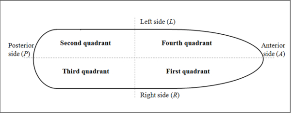
In line 4, UB2 divides the locations of the containership into four quadrants (see Figure 1). Each quadrant contains a subset of the locations which are formed by:
First quadrant: a set of anterior bays (A), right rows (R) and tiers of the ship. In particular, the set of bays A contains those bays which are in between 1 and ⌊I / 2⌋ and the set of rows R contains those rows whose index is odd.
Second quadrant: a set of posterior bays (P), left rows (L) and tiers of the ship. The set P is formed by the bays which are in between ⌊I / 2⌋ and I. The set L contains the rows with an even index.
Third quadrant: a set of posterior bays (P), right rows (R) and tiers of the ship.
Fourth quadrant: set of anterior bays (A), left rows (L) and tiers of the ship.
In the second phase (Lines 4 to 12), the algorithm tries to load containers into the containership. First, containers belonging to
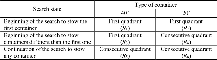
When the candidate location has been selected, we must verify that the assignation is feasible, that is, all the constraints involved in the problem must be satisfied. However, if the assignation is unfeasible, we try to allocate the container into a different quadrant. This quadrant is selected depending on the container type. On the one hand, for a 40' container, UB2 incrementally selects the next quadrant q+1, where q represents the number of the current quadrant (Rule
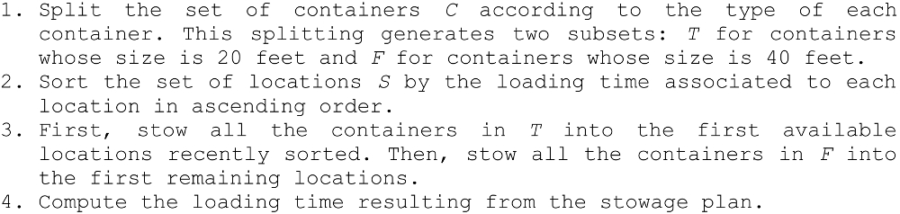
In the case of UB2 cannot allocate some containers into any quadrant, UB2 performs the last phase (Line 13). The last phase consists of firstly stowing the 40' containers into the available locations whose loading times are the highest. For the 20' containers, UB2 stows them into the remaining locations with the largest loading times. It is important to mention that in this phase UB2 does not consider the feasibility conditions.
Algorithm 3. Pseudocode of UB2.
5 Computational results
In this section, the performance of the proposed bounds is tested. In the following subsections, we describe the test instances, experimental environment and the computational analysis to evaluate the performance.
5.1. Test cases
In order to validate the proposed bounds, we used three sets of instances: A, B and C. The sets A and B have 24 instances each one, while the set C has 10 instances. Each test case (instance) is composed of four characteristic sets:
Sets of instances A and B share one characteristic: the tolerances. However, for set C, the set of pseudo-random instances 10, all the characteristics are different. We generate two different types of container for the sets A and B. Both of them were constructed according to the format and conditions defined in 1.
Tables 2, 3 and 4 report the containers characteristics of the sets A, B and C, respectively. Each table shows the total number of containers, expressed in TEU (Twenty-foot Equivalent Unit) and the absolute number (n); the numbers of containers whose type is 20' (T) and 40' (F), respectively; the number of containers for three classes of weight (L: low, M: medium, H: high); and the partition of containers by destination. Three classes of weight are considered, namely low (from 5 to 15 tons), medium (from 16 to 25 tons) and high containers (from 26 to 32 tons).
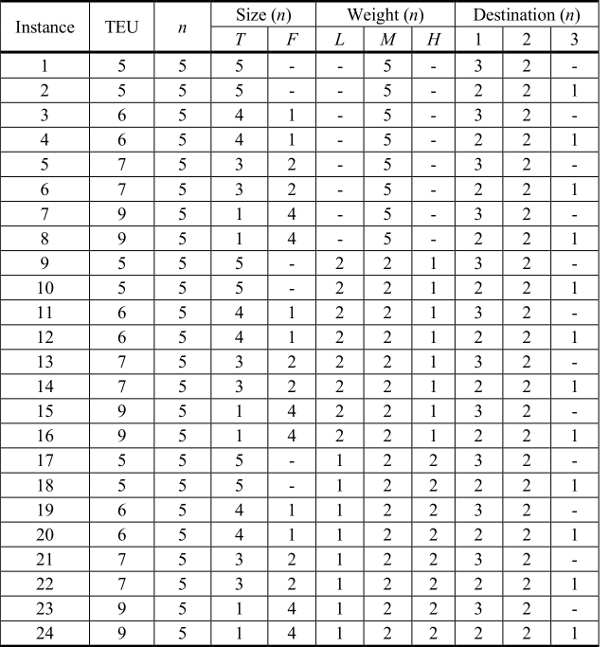
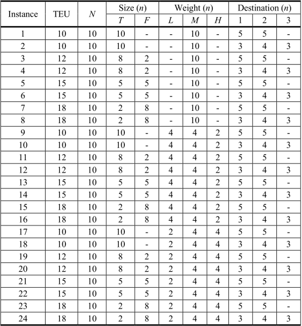

Regarding the containership characteristics, for the set of instances A, the hypothetical containership of small size has a maximum capacity of 24 TEUs. It is composed of 4 odd bays, 2 even bays, 2 rows and 3 tiers. In the set B the containership has a maximum capacity of 64 TEUs, 4 odd bays, 2 even bays, 4 rows and 4 tiers (2 in the hold and 2 in the upper deck, respectively). In the set C, the containership has a maximum capacity of 240 TEU. It is composed of 12 odd bays, 6 even bays, 4 rows and 5 tiers (3 in the hold and 2 in the upper deck, respectively).
The tolerances for the set of instances A and B are the following. Maximum horizontal weight tolerance (
Tables 5, 6, and 7 show the loading times for the containership corresponding to sets of instances A, B and C, respectively. The times are expressed in 1/100 of minute.


5.2. Experimental environment
The following configuration corresponds to the experimental conditions:
Software for general purpose: Operating system Microsoft Windows 7 Home Premium; Java programming language, Java Platform, JDK 1.6; and integrated development environment, NetBeans 7.2.
Software for optimization: solver CPLEX 12.5.
Hardware: Computer equipment with processor Intel (R) Core (TM) i5 CPU M430 2.27 GHz and RAM of 4 GB.
5.3. Computational analysis
The results of the performance of the proposed bounds are summarized in the Table 8. The structure of the table is the following. The first heading, Best known (BK), shows the average of the best known objective values and the average computing time required by CPLEX to solve a specific set of instances. It is worth to mention that the instances of the sets A and B were solved up to the optimality whereas the instances of the set C were stopped when the execution time reached 10 minutes. The next two headings, LB1 and LB2, present the performance of the proposed lower bounds. The last two headings, UB1 and UB2, report the performance of the proposed upper bounds. The attributes measured for the bounds are an average of: the objective values, the percentage of deviation and the computational time. The percentage of deviation for the lower bound and the upper bound is respectively computed by %LB = 100 - ((LB×100)/BK) and %UB = ((UB×100)/BK)-100, where BK stands for the best known value for a specific instance. The table has four main rows. The first three represent the sets of instances A, B and C. The last row shows the performance of the bounds over all the available instances.
Table 8 Comparison over sets A (24 instances), B (24 instances), C (10 instances) and all the instances (58).

*Average of the optimal solutions
From the experimental results we can observe the following: regarding the lower bounds, LB1 is faster than LB2 by 99.6%. However, LB2 seems to be better in the average quality of solutions for all instances. Specifically, LB2 outperforms LB1 by 4.5% in quality. We can also observe that the percentage of deviation for LB2 is less than that for LB1 by 54.3%. Furthermore, the percentage of deviation for LB1 is approximately 2.2 times greater than that for LB2.
With respect to the upper bounds, it can be seen that UB2 is better than UB1 in two of the attributes. More precisely, UB2 outperforms UB1 by 5.7% and 61.7%, in solution quality and percentage of deviation, respectively. The percentage of deviation for UB1 is approximately 2.6 times greater than that for UB2. Additionally, UB1 is faster than UB2 by 20.8% for all instances.
In order to determine the best combination of lower and upper bounds, we compute the gap, the time and the cost-benefit ratio between every pair of lower bound and upper bound. Table 9 summarizes the comparison of all the combinations. The measures are calculated using the last row (Overall) in Table 8. The first heading in Table 9 shows the gap (%Gap), which is computed by %Gap=(UB - LB) /UB×100. The second heading shows the average computing time (Time) that is computed by Time = (TimeLB + TimeUB )/2, where TimeLB and TimeUB are the average computing time required to compute the lower bound and the upper bound, respectively. Finally, the last heading shows a cost-benefit ratio (Ratio) to consider both the time spent and the quality obtained (1/Gap) by each combination. This ratio is calculated by Ratio = 1/(%Gap×Time). Thus, the larger the ratio value, the better the combination.

We can observe that the best combination is LB2 and UB2 considering the %Gap value. Regarding the computing time, the best combinations are LB1 with UB1 and LB1 with UB2. Notice that in both combinations LB1 appears. This is because LB1 is a deterministic procedure whose computational effort is relatively low. However, when measuring the cost-benefit ratio the best combination is LB1 and UB2.
6 Conclusions
In this paper the Master Bay Planning Problem (MBPP) was faced. When solving this kind of problems, an important issue is to develop good lower and upper bounds to reduce the search space of optimization algorithms. Therefore, we have proposed two new lower bounds, LB1 and LB2, and two new upper bounds, UB1 and UB2. Heuristics LB1, UB1 and UB2 are deterministic and easy to implement since they are constructed taking into account the problem characteristics. LB1 and UB1 are designed in such a way that their computational effort is low. Although UB2 is a more sophisticated procedure, it only requires a little bit more computational time to be executed. LB2 has good performance with respect to LB1. However, LB2 becomes slower as the size of the instance increases since it is based on a relaxation of the IP formulation.
We tested the performance of all the bounds with three sets of instances. Each lower and upper bound solved all the instances and the results were analyzed by computing the proximity to the best known objective values. The results clearly showed that the best lower bound is LB2 in solution quality and LB1 in computational time. UB2 outperforms UB1 in solution quality whereas UB1 is faster than UB2. When combining the lower bounds with the upper bounds, the best combination is LB2 and UB2 when considering only the Gap. Considering the computational time, the best combination is LB1 and UB1 since they bound each instance in 1 millisecond in average. These results indicate some tendencies which might not be conclusive since the attributes are analyzed independently. In order to consider both attributes together (Gap and Time), we propose to evaluate a cost-benefit ratio for each combination. The result of this analysis indicates that LB1 and UB2 is the best combination of lower bound and upper bound. They achieve the best compromise between quality and time.
Thus, through this research, we allow other researchers to select the best bounds according to their own objectives. For example, some researchers might be more interested in the quality of the solutions rather than the computational time spent or vice versa depending on the problem approached. Nevertheless, there might be some application problems in which the balance between quality and time is required. As a future work, it could be interesting to evaluate the impact of the proposed bounds in optimization algorithms.

