


 text new page (beta)
 English (pdf)
 Article in xml format
 Article references
 Send this article by e-mail
 Cited by SciELO
  Similars in
SciELO
Similars in
SciELO 
 Permalink
1 Introduction
Let G = (V, E) be a connected simple graph with n = |V| vertices and m = |E| edges. A linear ordering of the vertices is a bijection φ: V →{1,...,n} that assigns a different integer number between 1 and n to every vertex of G. It is easy to see that there are n! possible assignations for an n-sized graph. In fact, each assignation is a permutation of vertices and represents a feasible solution for the problem.
In order to formally define VSP, let us introduce the following definitions. Let φ(u) be the position of vertex u in solution φ. L(p,φ,G) = {u ϵ V |φ (u) ≤ p} represents the set of vertices placed to the left of fixed position p (with 1 ≤ p ≤ n). Symmetrically, R (p, φ,G) = {u ϵ V| φ (u) > p} is the set of vertices placed to the right of p. The set of vertex separators at p contains those vertices placed to the left of p with one or more adjacent vertices placed to the right of p, that is:
The number of vertices in δ(p,φ,G) is known as the cut value at position p. There are n cut values since there are n sets of vertex separators for each solution. The objective value of solution φ is given by the largest cut value and is formalized as follows:
The goal of VSP is to find the linear ordering with the minimum objective value out of all n! possible solutions 1. Unfortunately, finding such an ordering is very hard to achieve in practice since VSP is NP-hard 2. Even for special classes of structured graphs VSP remains NP-hard 3), (4), (5), (6. A structured graph has a characteristic and well-defined distribution of vertices and edges. Examples of this kind of graphs are trees or grids.
In the literature reviewed, we only found two methods to obtain the optimal objective value of VSP for generic graphs 7), (8. These methods are in the form of integer linear programming (IP) formulations. The first IP model represents the solution by permutation of vertices and generates
The main contribution of this research is the extension of the available exact methods for VSP with two new exact methods. In particular, we design a new IP formulation and an ad hoc branch and bound algorithm. Our IP formulation is actually an improvement of IP1. More precisely, we apply the compact linearization technique proposed by Liberti in 9 to linearize the binary product. This change of linearization technique allows us to reduce significantly the number of constraints by at least
The remainder of this paper is organized as follows. In Section 2 we present our proposed IP formulation, IPVSP. Our algorithm BBVSP is described in Section 3. The numerical experiment designed to evaluate our exact methods are reported in Section 4. Finally, in Section 5 we discuss the major findings of this research.
2 Integer programming formulation
In this section we describe our proposed integer linear programming formulation (IPVSP) for solving VSP. We start by describing the variables related to the model. We then present the mathematical formulation for IPVSP. Finally, we describe the purpose of each constraint and compare IPVSP with IP1 since IPVSP is an improvement of IP1 7.
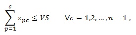
IPVSP uses one integer variable, VS, to compute the objective value of the current solution according to Equation (2). In addition, our formulation uses three types of binary variables, namely,
The total number of variables for IPVSP is
Subjet to:
 (4)
(4)
 (5)
(5)
 (6)
(6)
 (7)
(7)
 (8)
(8)
 (9)
(9)
 (10)
(10)
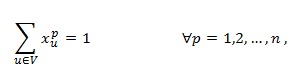
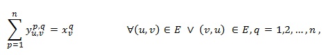
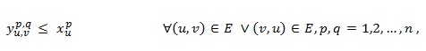
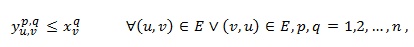
Assignment constraints (4) and (5) ensure that only feasible solutions are accepted. More precisely, they establish that each vertex u in the graph must be assigned only to one position p and each position must be only assigned to one vertex, respectively. The number of these constraints is 2n. Constraints (6) and (7) specify the connectivity of the graph in terms of the relative position of any pair of vertices u and v in the solution. Specifically,
As mentioned previously, the main difference between IP1 and IPVSP is the linearization technique applied. IP1 uses the traditional linearization technique, which produces the following three inequalities to the model:
 (11)
(11)
 (12)
(12)
 (13)
(13)
It is easy to see that the number of constraints generated by the traditional linearization technique is very large. Specifically, the linear subsystem (11) - (13) generates
3 Branch and Bound algorithm
In this section we present our branch and bound algorithm (BBVSP). We begin by describing the search tree in Section 3.1. Lower and upper bounds are presented in Section 3.2. We explain the branching and pruning strategies in Section 3.3. Section 3.4 presents an improvement of the traditional backtracking process. Finally, Section 3.5 presents our algorithm BBVSP. To avoid further confusions, we will refer to an element of the set V as vertex and to an element of the search tree as node.
3.1 The search tree
BBVSP models the solution space by means of a search tree in which every branch corresponds to a solution for VSP. The number of levels of the tree is n and the number of branches is n!. Each level corresponds to a position in the solution and each node of the tree is actually a vertex of the graph. Thus, when BBVSP visits a node at level p ( with 1 ≤ p≤ n), it means that BBVSP is assigning the visited node to position p of the solution. Each node at level p has n -p descendant nodes. The descendant nodes are those that are not in the branch at any level q (with 1 ≤ q ≤ p). Thus, each level of the tree has exactly n!/(n - p)! nodes. The total number of nodes in the search tree can be obtained by summing the number of nodes at each level of the tree. Specifically, there are
For practical purposes, the root of the tree is not considered a real node. The search tree shown in Figure 1 has n = 4 levels, 4! = 24 branches and
In order to visit all the solutions for an instance, BBVSP performs a depth-first-search (DFS) in the tree. BBVSP uses a last-in-first-out stack S as the main data structure and three additional data structures that improve the efficiency of the algorithm. All the structures used by BBVSP are described as follows.
S is an unbounded one-dimensional array which contains the nodes of the tree pending to be visited, that is, S is the active list of nodes. This is the main data structure of BBVSP.
Levels is a one-dimensional array of unbounded size which grows as S does. It records the level (in the search tree) of its corresponding node in S. Thus, the i-th element of Levels indicates the level of the i-th node in S.
Solution is a one-dimensional array of size n. It stores the visited nodes in the specific order. Thus, the node visited at level p is placed the p-th position of Solution.
Lower Bounds is a one-dimensional array of size n. It records the lower bounds of the nodes visited at previous levels. This avoids to unnecessarily re-compute the lower bound of a parent node and contributes to improve the efficiency of BBVSP. The i-th element of Lower Bounds is the cost of the i-th element of Solution.
3.2 Lower and upper bounds
A lower bound is a value associated to a particular node of the search tree and is used to indicate the cost of the node. When BBVSP visits a node, the lower bound of the node is computed in order for BBVSP to decide whether to continue exploring from the visited node or not. In this paper, we use the cut value [see Equation (1)] for computing the lower bound related to a node of the tree. The reason is simple, the cut value is a natural lower bound on the objective value of the solution [see Equation (2)].
When BBVSP visits a node at some level 1≤ p ≤ n, the nodes previously visited of the current branch are actually assigned to a specific position of the structure Solution. It means that these nodes must be in the set L(p,φ,G) at position p of the current solution. Thus, the elements of the set R(p,φ,G) are the remaining vertices, i.e., R(p,φ,G) = V\L(p,φ,G). Therefore, the lower bound of the node of level p can be obtained by computing |δ(p,φ,G)| according to Equation (1).
An upper bound is a value higher than the optimal value for an instance of VSP. At the beginning, BBVSP computes the upper bound of the instance by performing a constructive procedure named CVSP. This procedure allows BBVSP to considerably improve the efficiency since the number of nodes explored is reduced significantly. Moreover, when BBVSP finds an incumbent solution, its objective value becomes the new upper bound. The incumbent solution is defined to be the best feasible solution known so far during the search.
Let A and U be the sets of assigned and unassigned vertices, respectively. Initially, A = Ø and U = V. CVSP starts by assigning the vertex u ϵ U with the lowest (or the largest) adjacency degree to the first position of the solution. Then, the sets A and U must be properly updated, i.e., A = Aᴗ{u} and U = U \ {u}. For the rest of the procedure, the next vertex to be assigned is selected as follows. CVSP iteratively places all the unassigned vertices at the next available position p = |A| + 1 and keeps the vertex with the lowest (or the largest) cut value at p. More precisely, CVSP constructs the sets L(p,φ,G) = Aᴗ{u} and R(p,φ,G) = U \ {u} to compute c(u) = |δ(p,φ,G)| for all u ϵ U. Then, CVSP selects the vertex whose c-value is the lowest (or the largest) and updates the sets A and U by A = Aᴗ{v} and U = U \ {v}. The procedure finishes when all the vertices have been assigned, i.e., U = Ø. In case of ties, CVSP keeps the vertex whose lexicographical value is the smallest among the vertices involved in the tie. This makes CVSP a deterministic procedure.
It is easy to see that CVSP can be configured in four different ways based on the criteria to select the first vertex and the remaining vertices. In particular, CVSP1 uses the lowest degree criterion to select the first vertex and the lowest cut value criterion to select the next vertices. CVSP2 uses the lowest degree and the largest cut value criteria. CVSP3 uses the largest degree and the lowest cut value criteria. Finally, CVSP4 uses the largest degree and the largest cut value criteria.
3.3 Branching and pruning processes
Branching and pruning are perhaps the most important issues in the branch and bound algorithm. Branching allows the algorithm to discover new promising solutions that could lead to the optimal solution. Conversely, pruning avoids the solutions with no possibility of conducting to the optimum. It is easy to see that a mistaken design of these strategies could negatively affect the effectiveness of the algorithm since the optimum might not be found.
Let LB and UB represent the lower bound and the upper bound, respectively. When BBVSP visits an internal node (at level 1≤ p < n), the algorithm computes the lower bound of the node. If LB < UB then BBVSP performs the branching process, which consists of pushing the descendants of the node visited into the stack S in reverse lexicographical order. In addition, for each node entered into S, its corresponding level must be pushed into the structure Levels. Let us consider the search tree shown in Figure 1 to illustrate the branching strategy. Suppose that BBVSP is visiting node C from the first level and the algorithm decides to branch. Then, the nodes D, B and A must be pushed (in this order) into S and their corresponding levels 2, 2 and 2 must also be pushed into Levels.
The pruning process is performed when LB ≥ UB and consists of simply not performing the branching process. This is because all the solutions containing the nodes visited in the current branch will have an objective value of at least LB [see Equation (2)]. This implies that all of these solutions cannot be better than the current incumbent solution and hence visiting these solutions is actually a waste of time.
3.4 Improvement on the backtracking
When BBVSP is visiting a leaf node, that is the node at the last level (p = n), the objective value of the complete solution φ is computed. If the objective value improves the best objective value found so far (UB), then BBVSP updates both the incumbent solution and the upper bound, i.e., φ*←φ and UB←vs(φ*, G).
Afterwards, the algorithm must perform a backtracking process, which consists of going back to the parent node at previous level and continuing the exploration from it. Technically, the traditional backtracking (TBT) consists of simply popping the top element in S. Despite of its simplicity, this backtracking can be improved by taking advantage of the knowledge of the problem. More precisely, the improvement arose from the following observation. When BBVSP performs TBT, it unnecessarily explores unpromising nodes. This is because the position of the solution in which the lower bound is equal to the objective value is not always near to the leaves. In order to illustrate the previous observation, let us consider the example shown in Figure 2.
Fig. 2 A complete solution φ = (D,A,B,C,E,F,G,H) for a graph with eight vertices. The lower bound of each node is shown next to the node. The lower bounds of nodes C and E are equal to the upper bound. The leaf node H shows the objective value of the complete solution. The objective value becomes the new upper bound when it improves the previous upper bound.
As can be observed, BBVSP has reached a complete solution in which the nodes C and E (at levels 4 and 5, respectively) have a lower bound equal to the objective value (shown next to the leaf node H). If BBVSP performs TBT, then all the subtrees rooted from G, F, E and C must be explored since they are already in S. However, it is easy to see that exploring the aforementioned subtrees is not necessary since the new (current) upper bound is UB = 4. Therefore, no better solution can be found with the nodes D, A, B and C placed at the beginning of the permutation.
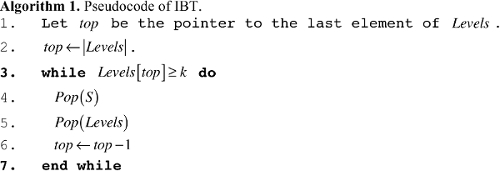
To overcome the previous issue, we propose to directly backtrack up to the node at level k - 1, where k represents the level of the first node (from the root to the leaves) whose lower bound is equal to the new upper bound. In our example, the first node whose lower bound is the upper bound is C at level k = 4. Therefore, BBVSP should backtrack up to the node B at level k - 1 = 3 to continue the exploration from the unexplored descendants of B (pending nodes E, F, G and H). We call this method improved backtracking (IBT). Technically, IBT consists of eliminating all the nodes in S whose levels are greater than or equal to level k. In addition, Levels must be properly updated. Algorithm 1 shows the pseudocode of IBT.
3.5 Algorithm BBVSP
BBVSP starts by computing the initial upper bound UB by executing the heuristic procedure CVSP described in Section 3.2. We have empirically determined the best configuration for CVSP in Section 4.3. The solution obtained by CVSP represents the initial incumbent solution, which is the best solution found so far. Then, BBVSP pushes the first pending nodes into S and their corresponding levels into Levels. The first nodes are all the vertices of the input graph and must be pushed in reverse lexicographical order to explore orderly the search tree since S is a last-in-first-out stack. The nodes of the first level of the tree constitute the roots of the main subtrees. All the nodes pushed into S are in the first level of the tree and hence Levels initially contains n numbers one.
When BBVSP visits some node of the tree, the lower bound LB of the node is computed to decide whether to continue the search in the current subtree or not. The computation of the lower bound was presented in Section 3.2. If LB < UB, BBVSP performs the branching process (see Section 3.3). Otherwise (LB ≥ UB), BBVSP prunes the current node and continues the search from the next pending node in S. When BBVSP reaches a leaf node, the objective value of the complete solution vs(φ,G) must be computed. If vs(φ,G) < UB, the upper bound and the incumbent solution must be updated and the backtracking process must also be performed. BBVSP uses the improved backtracking method presented in Section 3.4.
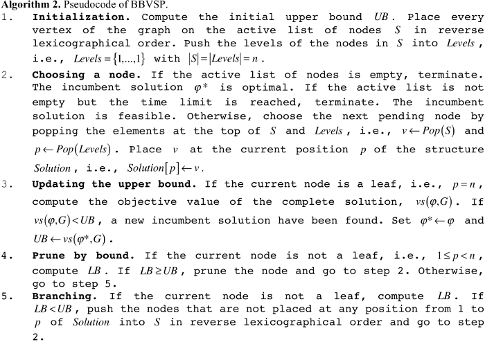
If all the nodes in the active list have been evaluated, i.e., S = Ø, BBVSP has found the optimal solution. This is the first criterion to stop the execution of our branch and bound. However, in some cases the size of the instance is relatively large and therefore another stopping criterion must be used. In particular, BBVSP uses the time limit as the second stopping condition. Thus, BBVSP finishes either when the active list of nodes is empty or when the time limit is reached. The pseudocode of BBVSP is presented in Algorithm 2.
4 Experiment and results
In this section we present the experiment conducted to assess the performance of both IPVSP and BBVSP. We have divided the experiment into two parts. The first part is intended to determine the best configuration for our constructive procedure CVSP. The second part evaluates our exact methods, IPVSP and BBVSP, and compares them with the best exact methods documented in the literature on VSP, IP1 and IP2.
4.1 Hardware and software platform
The experimental evaluation of the exact methods was conducted on a computer with an Intel Core 2 Duo processor (2.4 GHz) and 4 GB of RAM. All the methods were implemented in Java JRE 1.6.0_65. The IP formulations were solved by the well-known optimization engine CPLEX v12.5 10.
4.2 Test bed instances
In order to carry out the experiments, we use four types of instances, namely, GRID (5), TREE (15), HB (4) and SMALL (84). For each dataset, we have selected the smallest instances (with n ≤ 50) since we are dealing with exact methods. Thus, we have 108 instances to assess the performance of each method. The description of the datasets is the following:
GRID. This dataset consists of graphs of two-dimensional square meshes whose optimal value is known by construction. In particular, a square grid of size λ has an optimal value equal to λ. From this dataset, we only use five instances whose number of vertices ranges from 9 to 49 7.
TREE. From this dataset, we only use 15 trees whose optimal value is also known by construction. The number of vertices of the graphs used is 22 7.
HB. From this dataset, we only use 4 graphs. The optimal values of all the instances belonging to this dataset are not known. This dataset is considered the most difficult. The number of vertices of the instances selected ranges from 24 to 49 7.
SMALL. From this dataset, we use all the 84 instances. The optimal values of these instances are not known. The number of vertices of these instances ranges from 16 to 24 11.
4.3 First part of the experiment
The goal of this part of the experiment is to determine the most suitable variant of the constructive presented in Section 3.2, CVSP. As mentioned in the aforementioned section, there are four variants: CVSP1, CVSP2, CVSP3 and CVSP4. In order to determine the best variant, each one solved the entire dataset SMALL. As mentioned previously, all the variants are deterministic and hence they solve each instance once. Table 1 shows, for each variant of CVSP, the accumulated objective value (O.V.) and the accumulated execution time expressed in CPU seconds (Time).
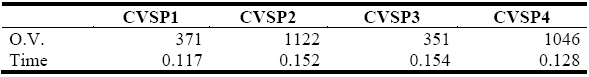
We can observe that the third variant, CVSP3, outperforms the other variants in solution quality. The execution time required by CVSP3 to solve all the instances is slightly larger than those of the other variants. Although CVSP3 recorded the largest accumulated execution time, this time is negligible when considering the execution time of the other variants. Consequently, we consider CVSP3 the best variant of CVSP and hence it will be coupled with BBVSP to compute the initial upper bound.
4.4 Second part of the experiment
The goal of the second part of the experiment is to assess the performance of the exact methods proposed and the exact methods available in the state-of-the-art. Specifically, IP1, IP2, IPVSP and BBVSP solved all the 108 instances. All the methods solved each instance either up to the optimality or up to the time limit. In particular, we considered a time limit of 300 CPU seconds for each instance. In some cases CPLEX was unable to find a feasible integer solution in the time limit. Thus, for those cases, we configured CPLEX to stop when the first feasible solution was found regardless of the time limitation. Table 2 presents the experimental results obtained for each exact method. The structure of the table is the following. The columns show the performance of each method: IP1, IP2, IPVSP and BBVSP. The rows are grouped by dataset and each group reports three statistics: the average objective value (O.V), the average computing time (Time) and the number of instances in which the method found the optimal solution (# Opt.).
Table 2 Final comparison of the exact methods IP1, IP2, IPVSP and BBVSP over all the 108 available instances.
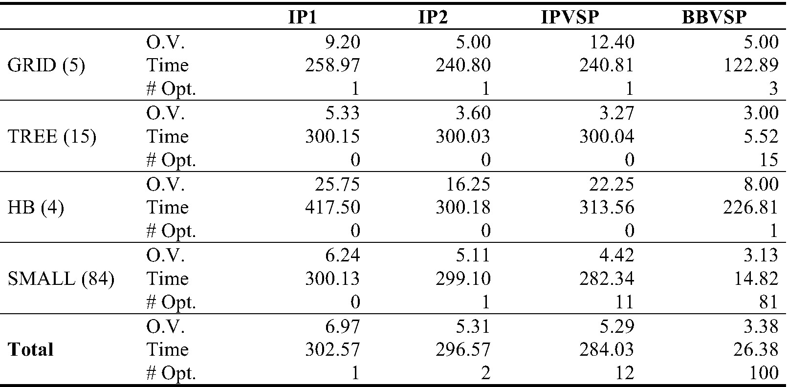
From the experimental results, we can observe that IP1 was the worst method since it obtained the largest average objective value for all the datasets. Moreover, IP1 only found one optimal solution (out of 108), which gives it an effectiveness of 0.9%. The computing time of IP1 was also the largest one, i.e., 302.6 seconds per instance in average. Notice that the average computing time of IP1 for dataset HB is quite large, i.e., 417.5 seconds. This is because CPLEX spent about 738 seconds to find the first feasible solution for one of the HB instances modeled by IP1.
As mentioned previously, IP2 is currently considered the best IP formulation for VSP. However, in this experiment IP2 was ranked number three in average objective value. IP2 found 2 optimal solutions out of 108 available instances, which gives it an effectiveness of 1.9%. It is important to point out that all the objective values found by IP2 for dataset GRID were the optimal values. Recall that the optimal values for datasets GRID and TREE are known by construction. However, these objective values were not quantified in the statistic # Opt since CPLEX did not finish its execution. Therefore, the optimality cannot be guaranteed. IP2 was also ranked number three in average computing time. In fact, there is a small difference between IP1 (the slowest method) and IP2 of 6 seconds and a larger difference between IPVSP (ranked number two in average computing time) and IP2 of 12.5 seconds.
Our IP formulation proposed, IPVSP, is the second best method in both quality and time. Specifically, IPVSP found 12 optimal objective values and hence it has an effectiveness of 11.1%. IPVSP was particularly effective in dataset SMALL, in which found 11 (out of 12) optimal values. Although the computing time of IPVSP was also the second best out of all the methods, there is a huge difference between BBVSP (the fastest method) and IPVSP of 257.65 seconds.
Our branch and bound algorithm proposed, BBVSP, emerges as the best method in both solution quality and computational time. In particular, BBVSP obtained the lowest average objective values, the largest number of optimal values found and the smallest amount of average computing time. More precisely, BBVSP found 100 optimal values out of 108 instances. This gives BBVSP a remarkable effectiveness of 92.6%. The average computing time of BBVSP was also impressive. BBVSP spent 26.4 seconds to solve an instance of VSP in average.
5 Conclusions
In this paper we have faced the vertex separation problem (VSP). In particular, we extend the available exact methods with one based on a new integer linear programming (IP) formulation (named as IPVSP) and the other based on the branch and bound methodology (named as BBVSP). IPVSP is an improvement of the IP formulation proposed by Duarte et al. in 7. The improvement consists of changing the technique applied to linearize the product of two binary variables. In particular, we use the compact linearization technique proposed by Liberti in 9. This allows us to reduce the number of constraints by at least 2mn2 , where n and m represent the number of vertices and edges of the graph, respectively. BBVSP uses an efficient constructive heuristic to obtain a tight initial upper bound and an improvement of the traditional backtracking process to prune unpromising nodes of the search tree.
We have conducted a numerical experimentation in order to assess the performance of our exact methods in practice. We compare our methods with the best exact methods for VSP in the literature, IP1 7 and IP2 8. The experimental results clearly show that BBVSP is the best exact method when considering both efficiency (time) and effectiveness (quality). More precisely, BBVSP achieved a remarkable effectiveness of 92.6%. This means that BBVSP solved 100 instances (out of 108) optimally. It is worth to mention that difference between BBVSP and the second best method (IPVSP) in effectiveness is huge, i.e., 81.5%. Additionally, BBVSP obtained the lowest average computing time. In particular, each instance was solved by BBVSP in 26.4 seconds in average, which represents a saving of time of about 91.3%, 91.1% and 90.7% with respect to IP1, IP2 and IPVSP, respectively. These results exhibit the importance of designing ad hoc algorithms. According to the results of the experiment, IPVSP is the best IP formulation for VSP. Specifically, IPVSP outperforms IP1 and IP2 by 10.2% and 9.2% in effectiveness, respectively.
Therefore, taking into account the data from the experiment, we can conclude that the approaches proposed in this paper were successfully applied since BBVSP and IPVSP outperforms the best exact approaches in the current state-of-the-art of VSP. All the methods and techniques proposed in this research can be easily adapted to other combinatorial optimization problems related to linear orderings such as cutwidth, sumcut, bandwidth or anti bandwidth.

