


Servicios Personalizados
Revista
Articulo
 texto en
  Inglés (pdf)
 Artículo en XML
 Referencias del artículo
 Enviar artículo por email
Indicadores
-
 Citado por SciELO
 -
 Accesos
Links relacionados
-
 Similares en
SciELO
Similares en
SciELO
Compartir

 Permalink
Revista mexicana de ciencias forestales
versión impresa ISSN 2007-1132
Rev. mex. de cienc. forestales vol.13 no.71 México may./jun. 2022 Epub 22-Ago-2022
https://doi.org/10.29298/rmcf.v13i71.1192
Research Article
Conservation of vegetation coverage in Maderas del Carmen, Coahuila, multitemporal analysis using SAVI index
1Facultad de Ciencias Biológicas, Universidad Juárez del Estado de Durango. México.
2Especies, Sociedad y Hábitat, A. C. México.
3Universidad Autónoma Agraria Antonio Narro. México.
4Naturaleza sin Fronteras. México.
Evidences of vegetation coverage management were analyzed according to Soil Adjusted Vegetation Index (SAVI) values in private and communal lands of the Maderas del Carmen and Ocampo Natural Protected Areas; the index values were generated from three Landsat satellite images of 1985, 2001 and 2019. The data index values were acquired from forests, scrublands, and grasslands from supervised classified maps generated with training areas, from Inegi vegetation and land use map series II, IV and VI, adding resources management intensity as a factor derived from property maps. A shapefile point network of the study area, with 500 m of separation, was created in order to capture the values of presence of forest, scrubland, or grassland ecosystems; the management intensity (Private lands with conservation, private lands with management, and communal lands with management) and the SAVI values from the three dates generated a database used to analyze the index values (vegetation coverage) through time. Normality tests were made in the database; no normal distribution was detected on them. The variance of the index was calculated by ecosystem and management factor (intensive, moderate and conservation). The results of the non-parametric H Kruskal Wallis tests indicated significant differences (α>0.95, Z = 2.394 critical value) on the three dates for all the ecosystems and management intensities. In the forests and grasslands, the private lands under conservation management exhibited the highest vegetation index values, while in the scrublands, the highest values corresponded to lands with a moderate management.
Key words Conservation; Index SAVI; Maderas del Carmen; forest management; multitemporal; Ocampo
Se analizaron evidencias de manejo en la cobertura vegetal, a partir de valores del Índice de Vegetación Normalizado de Suelo (SAVI) en terrenos privados y comunales de las áreas naturales protegidas Maderas del Carmen y Ocampo; los índices se generaron de tres imágenes de satélite Landsat de 1985, 2001 y 2019; los valores del índice se capturaron en áreas de bosque, matorral y pastizal de clasificaciones supervisadas obtenidas con áreas de entrenamiento usando las series II, IV y VI de Uso de Suelo y Vegetación de Inegi; y se agregó el factor manejo del recurso procedente de mapas prediales. En una red de puntos espaciada a 500 m dentro del área, se capturó la presencia de bosque, matorral y pastizal; la intensidad de manejo en terrenos privados (conservación y con manejo), así como terrenos comunales con manejo, además del valor del índice SAVI de tres fechas; con ello, se generó una base de datos para el análisis del comportamiento del índice (cobertura vegetal). Las pruebas de Chi cuadrada no detectaron una distribución normal. La varianza del índice se realizó por ecosistema y el factor de manejo (intensivo, moderado y de conservación). Los resultados indicaron diferencias significativas en la prueba H no paramétrica de Kruskal Wallis (α>0.95, Z = 2.394 valor crítico) en las tres fechas para todos los ecosistemas e intensidades de manejo. En bosques y pastizales los terrenos bajo manejo de conservación registraron los valores más altos de Índice de Vegetación; y en matorrales correspondió a los sitios de manejo moderado.
Palabras clave Conservación; índice SAVI; Maderas del Carmen; manejo; multitemporal; Ocampo
Introduction
The Maderas del Carmen region is a protected area declared since 1994. As an island-mountain, it is an important biological corridor for many migratory species (Miller et al., 2018); it includes remnant plant communities that constitute a refuge for various endemic taxa (Semarnat and Conanp, 2013). This region is located in the southeastern end of the Chihuahuan Desert ecoregion; its territory has mountain ranges that are isolated from the pine and oak forests ecoregion of the Eastern Sierra Madre (INEGI, Conabio, and INE, 2008).
Today, the vegetal cover can be rapidly monitored in large areas using remote sensing techniques, which are important tools for making estimates in fractions of the vegetation on large surface areas (Barati et al., 2011; Hansen et al., 2013). Remote sensing is also utilized in multi-temporal analyses in order to observe changes in the vegetal cover (Alencar da Silva et al., 2019), and monitor fires in order to generate risk maps (Brondi et al., 2016). In addition, vegetation indices such as NDVI are useful to detect the particular habitat conditions from which the movement of herbivorous wild animals is inferred (Pettorelli et al., 2011). The soil-adjusted vegetation index (SAVI) is used at a regional scale in semi-arid zones ―as it allows detecting changes in plant communities over multiple years― where seasonal vegetation and soil changes are usually minimized (White and Swint, 2014).
Spectral vegetation indices: Simple Ratio (SR), the Normalized Difference Vegetation Index (NDVI), and SAVI indicate a good correlation with vegetation changes, such as the Leaf Area Index (White and Swint, 2014). In turn, vegetation indexes are important in the derivation of parameters like the vegetal cover percentage (Gonzaga, 2015).
The forest cover and its degradation have been monitored in time series, using vegetation indexes (Schultz et al., 2018). The objective of the present study was to detect the changes in the vegetal cover of the mountain range, the hills, and the plains that make up the Maderas del Carmen region of Coahuila State over the last few decades, in three of its main ecosystems subjected to various management intensities. The analysis was carried out considering a monitoring of values of the SAVI vegetation index in each ecosystem.
Materials and Methods
Study area
The research was carried out in the area located between Maderas del Carmen and Ocampo Natural Protected Areas, both included in the Wildlife Protection Area (WPA) category (Conanp, 2016). The study area encompasses part of the Acuña, Múzquiz and Ocampo municipalities in the northeast of the state of Coahuila (Figure 1).

Acquisition and processing of satellite images
Satellite images available from the Landsat programs for the years 1985, 2001 and 2019 were located and downloaded from the Global Visualization platform of the U. S. Geological Survey (GloVis, 2005). Other images, for the 1986, 2002 and 2020 years, were also obtained, all of them in a 30 X 30 m spatial resolution. Images of the rainy season were also incorporated including the red and infrared bands: b3 and b4 from the 1980´s Landsat 5 and from Landsat 7 of the beginning of 2000, and b4 and b5 from the 2019 Landsat 8, in which the following characteristics converge: the lowest possible percentage of cloudiness and no default remote sensing scanning to confirm the graphic tendencies in the calculated index, or identify inconsistencies or lack of data for the rainy season, between August and October.
The season of the images was selected with the expectation of the maximum spectral response as a result of the annual growth of the vegetation. The selection of the season of the year for the images was made expecting the maximum spectral response due to the annual growth of the vegetation. In addition, the WorldClim 2.1 database of historical monthly climate data of 1970-2000 was consulted (Fick and Hijmans, 2017). The variables utilized were the monthly mean temperature (°C) and the monthly precipitation (mm).
The dates September 24th, 1985, October 14th, 2001, and October 8th, 2019 were selected based on this analysis. An atmospheric correction was applied to all bands. Compound images were created to include the red and the near infrared bands according to the platform and sensor of each image. The plots located in the WFA Maderas del Carmen and Ocampo were selected, based on the property files of the region in order to generate a range polygon of the area of interest, in which a 1 000 m buffer was generated in order to in order to crop the three satellite images (Figure 1).
Supervised classifications
In terms of the different times elapsed between the three images and in order to generate three training areas in the supervised classifications, the thematic vectorial covers of the National Institute of Statistics and Geography (Instituto Nacional de Estadística y Geografía, Inegi) regarding the Soil Use and Vegetation (1:250 000) were utilized as a base and reference for selecting sample polygons as spectral signatures of the various types of vegetation or ecosystems; series II for the 1985 image, series IV for the 2001 one, and series VI for the training areas of the 2019 image. The soil use and vegetation types corresponded to the Inegi series: forests (all their variants and combinations, including chaparral), microphytic and rosetophyle scrubs, grasslands (natural, induced, and halophytic), rocky surface area (bedrock and alluvium), and surface with water (permanent rivers and small dams).
Recodings were performed at the ecosystem level in order to obtain forest, scrubland, and grassland areas. The coding of sample polygons used as a spectral signature was utilized in the digital classification processes. The ArcGIS 10.8.1 image classification module of ESRI© 2020 was utilized to classify the three images with the Maximum Likelihood Supervised Classification method. For this purpose, a unique set of spectral signatures was edited and used for each processed date.
Post-classification processes
Once the classification and the soil use and vegetation map were generated for each date, with the initially assigned class names from the utilized training areas preserved in each map, the original classes were visually validated with Google Earth Pro and with two visits to the study area during the summer of 2020, in addition to a previous knowledge of the site since the year 2000. The results were vectorized in order to generate shapefiles that preserved a field with the name of the class used as training. Additional fields with the name and the ecosystem made a revision and a reclassification possible, in which the generated spectral signatures were recoded to the types of soil use and vegetation created according to the assigned classes.
Once the vegetation types and ecosystems were validated for each date, the three dominant ecosystems in terms of landscape level coverage in the area were analyzed, and the areas were calculated in square kilometers for the three dates, in order to analyze the changes between 1985, 2001 and 2019.
In order to ensure the recording of the vegetation index values calculated for all ecosystems over the time considered, the three vegetation maps were intersected through a geoprocess in order to locate those areas with permanence of the three most widely distributed vegetation types ―forests, scrublands and grasslands―, and thus the calculated values of the SAVI index between 1985 and 2019 were recorded. This made it possible to register the change in values during the period and to interpret their cover.
Use of the SAVI index
In each original image cropped to the boundaries of the study area, the R (red) and NIR (near infrared) bands of each date were used in the generation of the SAVI index with the Map Algebra module of Quantum GIS© 3.16 (QGIS Development Team, 2020); vegetation indexes were generated for each satellite image (Landsat 1, 2, 5 or 8, depending on the date) and band number (b) of the electromagnetic range corresponding to the red (R) and near infrared (NIR) bands to estimate the Soil Adjusted Vegetation Index (SAVI). Formula (1) was applied in order to calculate the index for each date.
Where:
R = Red band.
NIR = Near infrared band.
L = Constant value of 0.5 for soils in vegetation considering a semi-arid and temperate climate in the region (White and Swint, 2014).
Classified vegetation types (ecosystem) and plots with different management intensities in the study area
The total area analyzed is 2 800 km2; 50.8 % of it are subjected to diverse management activities, while the remaining 49.2 % have been under conservation since 2000. There is a detailed background of vegetation classification (Muldavin et. al., 2004) considering up to 33 plant associations grouped into five communities. However, in order to simplify this study regarding the analysis of vegetation types, and given that the difference in spectral response is considered to be greater as the cover increases at the ecosystem level, the results of each classification were based on the location of training areas used as a sample of the main ecosystems existing in the area, according to the Land Use and Vegetation series II and VI of Inegi (INEGI, 2001; INEGI, 2016), in which six land uses and vegetation were identified, some in secondary condition ―verified through field visits and Google Earth―, by direct observation of the polygons of the training areas.
As a post-processing step, all polygons smaller than 10 000 m2 (1 ha) were eliminated in order to avoid the "salt and pepper" effect. Subsequently, the polygons were reclassified into three major generalized ecosystems. In the reclassified and vectorized maps resulting from these classifications, the three most extensive and widespread ecosystems ―forests, scrublands, and grasslands― were identified.
Finally, based on a vector file with the zone's property boundaries and on the consultation of the property regime, plots with ejido community management, private plots with livestock management, and private lands without livestock and with conservation vocation since 2000 were recognized. A field was added to the database for the type of management, divided by intensity of use. The type of management was captured in the property file and intersected with the ecosystem polygons for each of the three dates analyzed, so that maps indicating ecosystems and management type were generated for 1985, 2001 and 2019.
Capture of SAVI index values by ecosystem and management regime
Within the distribution area of the three classified ecosystems, a point type shapefile was made on a grid pattern, systematically divided every 500 m using the Repeating Shapes module for ESRI (Jenness, 2012). The SAVI index values corresponding to the three dates analyzed were captured in the shapefile thus created, and the ecosystem and management regime records were kept using the Extract Multi Values to Point module of ArcGIS 10.8 (ESRI, 2020). Thus, a database of 22 250 records was generated with the UTM coordinate of each specific record in the study area. The base arrangement was organized using the SAVI index values for three dates as the main variable, and the ecosystem factors (forest, scrubland and grassland areas), and a management factor (conservation areas, private areas with traditional management and communal ejido areas with extensive exploitation). The methodological scheme is described in Figures 2a and 2b.
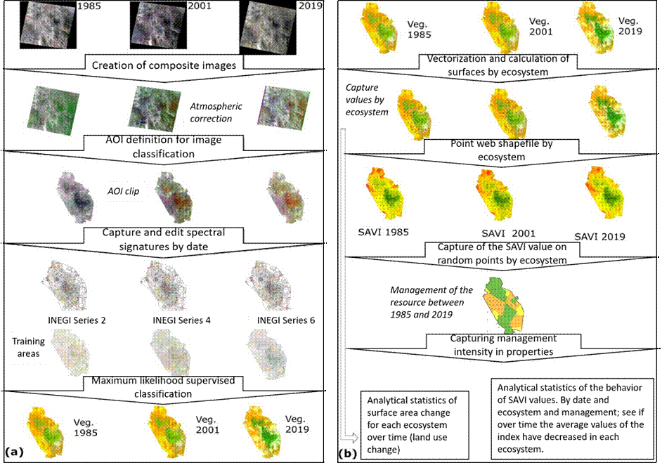
Figure 2 (a) Methodological scheme of preprocessing and digital classification of Landsat images of the study area, acquisition, atmospheric correction, cropping, composite images, training areas and supervised classification; (b) Verification and recoding of classes by ecosystem and generation of a network of points to capture these values and ecosystem and management factors.
Statistical data analysis
The resulting database was converted to a DBF vector file format from the shapefile to Excel. Each of the columns was identified with a representative name, and the data was separated by ecosystem for analysis through filtering, and the intensity of management by ecosystem in databases separated by date was left as a factor for comparison analysis, in order to test for normality. The mean values by ecosystem and date were plotted to observe the trend over time. Normality tests were performed using Pearson's Chi-square test with R Commander of R© (Fox, 2020) for SAVI ecosystem and management data on all three dates. When normality was not observed in the distribution of the data for the analysis of variance, the Kruskal Wallis H-test was applied to determine differences between the means of each management intensity in the three ecosystems and the three dates, using the Statistix 8.1 package (Statistix, 2003).
The results were concentrated by ecosystem and date to analyze differences between the means of each management intensity by ecosystem and to determine in which ecosystem there was greater coverage, based on the mean value of the index.
Results
Spatial analysis of ecosystems and tendencies between 1985 and 2019
According to the results of the supervised and recoded classification at the ecosystem level, of the three main ecosystems in the area, forests have had a spatial reduction of just over 300 km2 between 1985 and 2019. The areas of scrubland have exhibited only minor changes, decreasing by approximately 4 km2 between 1985 and 2019. On the other hand, grasslands have increased by almost 3 600 km2 over a 34-year period (Figure 3a).

Tendencies in SAVI index values
The average values of the SAVI index calculated for forest areas showed a gradual decline from 1985 until 2002, when the value began to recover, until 2020; the values were always higher for the managed private areas dedicated to conservation, while privately lands under management exhibited intermediate values. Finally, the ejidos registered the lowest index values on all dates (Figure 3b).
In scrublands, a gradually decreasing trend was observed from 1985 to 2002, with an increase in 2019; the highest values corresponded to the land under conservation management at the beginning of the period and towards the end, with similar figures in the years 2002 and 2019; private farms with management registered the lowest values during the entire period analyzed, while community-managed lands had intermediate values between those of private lands and areas with conservation status (Figure 3c).
The grasslands exhibited a similar tendency to that of the forests and scrublands, with a gradual decrease in values between the 1980´s and the beginning of the 21st century, with an increase after 2002. In this ecosystem, the lands dedicated to conservation did not have higher index values. The highest values were obtained from 2002 to 2020. Among the grasslands, managed private plots registered the highest SAVI indexes but have exhibited intermediate values in the last 20 years. Finally, the areas with communal management had a general constant of similarly low vegetation indexes from the beginning of 2001 to 2002, and in the final years of the study they exhibited the lowest SAVI index among the different property regimes (Figure 3d).
Data normality tests
In the analyzed years, between 1985, 2001 and 2019, all the mean SAVI values for the three main ecosystems yielded lower probability values than the Pearson Chi-square p-values calculated for forests (41.6-105.3), scrublands (431.9-2 078), and grasslands (231.9-2 342); i.e., there was no normality in data distribution (with p-values of 0.032 to 2.2e-16).
Management factor in the forest ecosystem
According to the non-parametric analysis of variance in the Kruskal-Wallis H-test, in 1985 there were significant differences (α=0.05; critical value Z=2.394) between private plots with conservation management, private plots with management, and ejidos. The first had the highest value, followed by the private plots with management, and the ejidos had the lowest average index value. In 2001, there were differences between private conservation and managed plots and land under communal management (α=0.05, critical value Z=2.394); communal management presented the lowest index value. In 2019, both managed and conservation private plots differed from ejidos according to the H-test (α=0.05, critical value Z=2.394); the lowest value corresponded to the plots under community management (Table 1).
Table 1 Mean comparison of SAVI values, H Kruskal Wallis test (α=0.05) in three management intensities of three ecosystems in the study area from 1985 to 2019.
| 1985 | 2001 | 2019 | |||||||
|---|---|---|---|---|---|---|---|---|---|
| Ecosystem / Management |
Private conserv. |
Private managem. |
Community managem. |
Private conserv. |
Private managem. |
Community managem. |
Private conserv. |
Private managem. |
Community managem. |
| Forest | A | B | C | A | A | B | A | A | B |
| Scrubland | A | B | C | B | C | A | A | A | A |
| Grassland | A | B | B | C | A | B | A | B | B |
Equal letters indicate equal statistical significance.
Management factor in the scrubland ecosystem
In scrublands, the non-parametric analysis of variance in the 1985 Kruskal-Wallis H-test indicated significant differences (α=0.05; critical value Z=2.394) between private land with conservation management, private land with management and ejidos; from these, the first exhibited the highest value, followed by the private plots with management, and the lowest average index value was estimated in the ejidos (Table 1). Significant differences persisted in 2001 (α=0.05, critical value Z=2.394) between the three types of management; the lands with the highest values were those under community management, followed by private lands under conservation management, while private lands under management had the lowest average value. In 2019, there was a change, and no significant differences were detected between management intensities for the scrublands (α=0.05, critical value Z=2.394) (Table 1).
Management factor in the grassland ecosystem
The non-parametric analysis of variance of the Kruskal-Wallis H-test showed significant differences for 1985 in the grasslands (α=0.05; critical value Z=2.394) between private lands under conservation management and private lands under management and ejidos; the former had the highest value, followed by the private plots with management, and the ejidos had the lowest average index (Table 1). In 2001, there was a significant difference between the three management intensities according to the Kruskal Wallis H-test (α=0.05; critical value Z=2.394); in this case, private plots with management exhibited the highest value, followed by the ejidos, while the plots under conservation management had the lowest rate (Table 1). In 2019, the situation changed because significant differences were detected by the H-test (α=0.05; critical value Z=2.394); the areas with conservation management registered the highest value, followed by privately managed land and community-managed plots, which were statistically equal, below the other two management types (Table 1).
Discussion
The period selected for classification and mapping of the ecosystems (September-October) was appropriate, despite the rainy season in this mountainous and hillside area, since the images showed sparse to no cloud cover; it also exhibited growth of foliage in response to the precipitation received at that stage of the year and in the months of the rainy season.
The vegetation index used (SAVI) was better than an NDVI calculation, since other studies indicate 28 % error in the NDVI for light and dry soils, while the error percentage for SAVI is 12 % in the same soils; around 50 % in scrublands, and 20 % in grasslands, i.e., desert ecosystems with light, dry soils (Gonzaga, 2015; Vani and Mandla, 2017). On the other hand, certain adjusted soil indexes such as SAVI have similar accuracies to that of NDVI´s (Barati et al., 2011).
The forest ecosystem shows a spatial decrease in its surface area; the wooded areas in the 1980´s were estimated to cover more than 800 km2 and in recent years they occupied 527 km2; this rate of loss is not so much due to forest harvesting, which has not been permitted since the late 1990´s (Semarnat and Conanp, 2013). In the Ocampo APFF, forest harvesting is for self-consumption (Semarnat and Conanp, 2015); therefore, the changes may be due to recurrent fires in the area (Brondi et al., 2016) that have given rise to a change from pine or pine-oak forests to low, somewhat open oak groves (Alanís et al., 2014) ―equivalent to chaparral in the classification by INEGI―, which then become integrated into grasslands in the higher parts, and into rosette scrubs in the lower parts.
According to the vegetation index values, the best preserved sites were located
on private land under conservation management, exhibiting the highest SAVI
values (
The plots in the scrubland ecosystem exhibited little spatial change in the
analyzed period; the range of SAVI values in managed areas with conservation was
The surface area of the grasslands increased, possibly due to changes in
degradation in the border zone with forests and scrublands; in private plots
with conservation, the index values were
According to the mean comparisons (Table 1), the tendencies observed indicate that during the entire stage of the analysis, private plots with conservation use had the highest vegetation index values in forested areas. The same situation is observed in the scrublands and grasslands, with a change at the end of the 20th century, when the vegetation index values registered were not high, equaling those of private plots under exploitation; however, these values improved in 2019 and 2020. These tendencies of the vegetation cover to degrade or recover as an effect of management have been detected thanks to the monitoring of the vegetation index values (Vani and Mandla, 2017; Xiao et al., 2017).
Conclusions
The SAVI index values indicate a change in the vegetation cover ―an effect that is manifest in the amount of bare soil present in each community, along with the intensity of management; this is mainly observed in the forest ecosystem, which has been limited in recent years.
The forest areas in Maderas del Carmen have a gradually increasing cover loss rate, historically reflected in the vegetation index values until the end of the 20th century, and show a marked conservation process, mainly in the private plots dedicated to its conservation since 2002.
In the shrublands, there is no significant spatial decrease over time, although their average SAVI index values, and therefore, their vegetation cover, are below those of the grasslands. Conservation plots in the scrub ecosystem have higher average values, corresponding to a higher ground cover, than other scrublands in the community-managed ejidos and in private plots under management.
The grasslands have exhibited an increase in geographic area in recent years, where private plots have continuously had a higher average vegetation index value than that estimated for communal lands. In 2002, private lands dedicated to conservation improved their coverage, compared to the rest of the managed areas; this is made evident by the higher SAVI values observed in the last 20 years.
Acknowledgments
The authors wish to express their gratitude to Naturaleza sin Fronteras A. C., for having favored the field visits and allowed the use of the facilities of the El Carmen Reserve, the site of the research between 2020 and 2021, and to the School of Biological Sciences of the Juárez University of the State Durango (Universidad Juárez del Estado de Durango), Gómez Palacio campus, for having supported our research.
REFERENCES
Alanís R., E., J. Jiménez P., M. A. González T., E. J. Treviño G., O. A. Aguirre C., J. I. Yerena Y. y J. M. Mata B. 2014. Efecto de los incendios en la estructura del sotobosque de un ecosistema templado. Revista Mexicana de Ciencias Forestales 5(22):74-85. Doi: 10.29298/rmcf.v5i22.351. [ Links ]
Alencar da Silva, A., K. M., M. C. Parodi D., R. Silva. N. y D. Opazo A. 2019. Variabilidad espacial y temporal de la cobertura vegetal de los años 1984 a 2011 en la Cuenca hidrográfica del Río Moxotó, Parnambuco, Brasil. Diálogo Andino 58:139-150. Doi: 10.4067/S0719-26812019000100139. [ Links ]
Barati, S., B. Rayegani, M. Saati, A. Sharifi and M. Nasri. 2011. Comparison the accuracies of different spectral indices for estimation of vegetation cover fraction in sparse vegetated areas. The Egyptian Journal of Remote Sensing and Space Sciences 14(1):49-56. Doi: 10.1016/j.ejrs.2011.06.001. [ Links ]
Brondi R., N. F., F. X. Lasso G. y A. Espinosa T. 2016. Mapeo del índice de peligro de incendio forestal en el bosque de coníferas del Área Natural Protegida de Flora y Fauna: Maderas del Carmen, Coahuila. Industrial Data 19(1):78-88. Doi: 10.15381/idata.v19i1.12540. [ Links ]
Comisión Nacional de Áreas Naturales Protegidas (CONANP). 2016. Áreas protegidas decretadas. Ciudad de México: Secretaría de Medio Ambiente y Recursos Naturales. http://www.conabio.gob.mx/informacion/gis/ . Descarga en: Regionalización (172), Bióticas (69). (fecha de consulta 3 de mayo de 2021). [ Links ]
Environmental Systems Research Institute (ESRI). 2020. ArcGIS Desktop: Release 10. Environmental Systems Research Institute. Redlands, CA., USA. [ Links ]
Fick, S. E. and R. J. Hijmans. 2017. WorldClim 2: new 1km spatial resolution climate surfaces for global land areas. International Journal of Climatology 37(12):4302-4315. Doi: 10.1002/joc.5086. [ Links ]
Fox J. 2020. The R Commander: A basic-Statistics GUI for R Current Version 2.7-1, 7-1, https://socialsciences.mcmaster.ca/jfox/Misc/Rcmdr/ (10 de febrero de 2021). [ Links ]
GloVis. 2005. Global Visualization (GloVis) Viewer. U. S. Department of the Interior, U. S. Geological Survey. https://glovis.usgs.gov/ . (5 de mayo de 2021). [ Links ]
Gonzaga A., C. 2015. Aplicación de índices de vegetación derivados de imágenes satelitales para análisis de coberturas vegetales en la provincia de Loja, Ecuador. CEDAMAZ 5(1):30-41. https://revistas.unl.edu.ec/index.php/cedamaz/article/view/43 (14 de junio de 2021). [ Links ]
Hansen, M. C., P. V. Potapov, M. Moore, M. Hancher, S. A. Turubanova, A. Tyukavina, D. Thau, S. V. Stehman, S. J. Goetz T. R. Loveland, A. Kommareddy, A. Egorov, L. Chini, C. G. Justice and J. R. G. Townshend. 2013. High-resolution global maps of 21st-Century forest cover change. Science 342(6160):850-853. Doi: 10.1126/science.1244693. [ Links ]
Instituto Nacional de Estadística y Geografía e Informática (INEGI) y Comisión Nacional para el Conocimiento y Uso de la Biodiversidad (CONABIO) e Instituto Nacional de Ecología, (INE). 2008. Ecorregiones terrestres de México. http://www.conabio.gob.mx/informacion/gis/ . Descarga en: Regionalización (172), Bióticas (69). (14 de mayo de 2021). [ Links ]
Instituto Nacional de Estadística, Geografía e Informática (INEGI). 2001. Uso del suelo y vegetación, escala 1:250 000, serie II (continuo nacional). Descarga en: Vegetación y uso del suelo (65) INEGI (7). http://www.conabio.gob.mx/informacion/gis/ . (12 de mayo de 2020). [ Links ]
Instituto Nacional de Estadística, Geografía e Informática (INEGI). 2016. Uso del suelo y vegetación, escala 1:250 000, serie VI (continuo nacional). Descarga en: Vegetación y uso del suelo (65), INEGI (7). http://www.conabio.gob.mx/informacion/gis/ . (12 de mayo de 2020). [ Links ]
Jenness, J. 2012. Repeating Shapes. Jennes Enterprises. Flagstaff, AZ., U. S. A. http://www.jennessent.com/arcgis/repeat_shapes.htm . (23 de mayo de 2020). [ Links ]
Miller E., T., J. E. McCormack, G. Levandoski and B. R. McKinney. 2018. Sixty years on: birds of the Sierra del Carmen, Coahuila, Mexico, revisited. Bulletin of the British Ornitologist Club. 138(4):318-334. Doi: 10.25226/bboc.v138i4.2018.a4. [ Links ]
Muldavin, E. H., G. Harper, P. Neville and S. Wood. 2004. A Vegetation Classification of the Sierra del Carmen, U. S. A. and México. In: Hoyt, C. A. and J. Karges (editors). Proceedings of the Sixth Symposium on the Natural Resources of the Chihuahuan Desert Region. Chihuahuan Desert Research Institute. Fort Davis, TX., U. S. A. pp. 117-150. http://www.cdri.org/uploads/3/1/7/8/31783917/final_chapter_9_muldavin.pdf . (10 de febrero de 2021). [ Links ]
Pettorelli, N., S. Ryan, T. Mueller, N. Bunnefeld, B. Jędrzejewska, M. Lima and K. Kausrud. 2011. The Normalized Difference Vegetation Index (NDVI): unforeseen successes in animal ecology. Climate Research 46:15-27. Doi: 10.3354/cr00936. [ Links ]
QGIS Development Team. 2020. QGIS Geographic Information System. Open Source Geospatial Foundation Project. http://qgis.org (20 de junio de 2020). [ Links ]
Secretaría del Medio Ambiente y Recursos Naturales (Semarnat) y Comisión Nacional de Áreas Naturales Protegidas (Conanp). Programa de Manejo Área de Protección de Flora y Fauna Maderas del Carmen. Comisión Nacional de Áreas Naturales Protegidas. Tlalpan, México D. F., México. 156 p. [ Links ]
Secretaría del Medio Ambiente y Recursos Naturales (Semarnat) y Comisión Nacional de Áreas Naturales Protegidas (Conanp). 2015. Programa de Manejo Área de Protección de Flora y Fauna Ocampo. Comisión Nacional de Áreas Naturales Protegidas. Miguel Hidalgo, México D. F., México. 164 p. [ Links ]
Statistix 8.1. 2003. User’s Manual. Analytical Software, Tallahassee. Analytical Software. PO Box 12185. Tallahassee, FL., U. S. A. 396 p. ISBN 1-881789-06-3. [ Links ]
Schultz, M., A. Shapiro, J. G. P. W. Clevers, C. Beech and M. Herold. 2018. Forest cover and vegetation degradation detection in the Kavango Sambezi Transfrontier Conservation Area Using BFAST Monitor. Remote Sensing 10(11):1850. Doi: 10.3390/rs10111850. [ Links ]
Vani, V. and V. R. Mandla. 2017. Comparative study of NDVI and SAVI vegetation indices in Anantapur district semi-arid areas. International Journal of Civil Engineering and Technology 8(4):559-566. https://iaeme.com/MasterAdmin/Journal_uploads/IJCIET/VOLUME_8_ISSUE_4/IJCIET_08_04_063.pdf . (25 de agosto de 2021). [ Links ]
White, J. D. and P. Swint. 2014. Fire effects in the northern Chihuahuan Desert derived from Landsat-5 Thematic Mapper spectral indices. Journal of Applied Remote Sensing 8(1):083667. Spectral indices. Doi: 10.1117/1.JRS.8.083667. [ Links ]
Xiao, Q., J. Tao, Y. Xiao and F. Qian. 2017. Monitoring vegetation cover in Chongqing between 2001 and 2010 using remote sensing data. Environmental Monitoring and Assessment 189(10):493. Doi: 10.1007/s10661-017-6210-1. [ Links ]
Received: July 26, 2021; Accepted: April 20, 2022
 Este es un artículo publicado en acceso abierto bajo una licencia
Creative Commons
Este es un artículo publicado en acceso abierto bajo una licencia
Creative Commons
