Spatial distribution of fuel loads in a pine-oak sample plot

Chávez Durán, Álvaro Agustín; Bustos Santana, Abundio; Chávez Durán, Héctor Manuel; Mora Orozco, Celia De la; Flores Garnica, José Germán; Rubio Camacho, Ernesto Alonso; Xelhuantzi Carmona, Jaqueline; Chávez Durán, Álvaro Agustín; Bustos Santana, Abundio; Chávez Durán, Héctor Manuel; Mora Orozco, Celia De la; Flores Garnica, José Germán; Rubio Camacho, Ernesto Alonso; Xelhuantzi Carmona, Jaqueline

doi:10.29298/rmcf.v12i65.787

Services on Demand

Journal

Article

Indicators

Cited by SciELO
Access statistics

Revista mexicana de ciencias forestales

Print version ISSN 2007-1132

Rev. mex. de cienc. forestales vol.12 n.65 México May./Jun. 2021 Epub Aug 30, 2021

https://doi.org/10.29298/rmcf.v12i65.787

Scientific article

Spatial distribution of fuel loads in a pine-oak sample plot

Álvaro Agustín Chávez Durán¹^*

Abundio Bustos Santana²

Héctor Manuel Chávez Durán³

Celia De la Mora Orozco¹

José Germán Flores Garnica¹

Ernesto Alonso Rubio Camacho¹

Jaqueline Xelhuantzi Carmona¹

^¹Instituto Nacional de Investigaciones Forestales, Agrícolas y Pecuarias. CIR Pacífico Centro. Campo Experimental Centro Altos de Jalisco. México.

^²Tecnológico Nacional de México. Ingeniería en Innovación Agrícola Sustentable. México.

^³Universidad de Colima. Facultad de Ingeniería Mecánica y Eléctrica. México.

Abstract

Forest fires are an ecological factor of high importance in ecosystems. A forest fire requires forest fuel, favorable environmental conditions and a starting factor in order to occur. Forest fuels are considered the core element in fire management since they are the only ones that can be handled and thus, modify their influence on fire behavior. The purpose of the present work is to show the variability and spatial distribution of dead fuel loads in a pine-oak forest plot with a surface area of one hectare. Field evaluations were used as a data collection technique, and geostatistical methods, as analysis tools. The general average of the fuel loads was 54.86 Mg ha^-1, with load areas larger than 100 Mg ha^-1. Moreover, high spatial variability and independence of the fuel components were identified, with load differences up to 116.61 Mg ha^-1 at only 72.11 m of distance. This work is envisioned as an important basis for studies of fuel loads at a highly detailed level. This will allow operational areas and decision makers to streamline the transition process towards fire management.

Key words: Fuels; fire behavior; distribution; fire; independence; fire management; spatial variability

Resumen

Los incendios forestales son un factor ecológico de gran importancia en los ecosistemas. Para que un incendio forestal ocurra se requiere de material combustible, condiciones ambientales favorables y un factor de inicio. Los combustibles forestales son considerados el elemento núcleo en el manejo del fuego, ya que son los únicos que pueden manipularse y así, modificar su influencia en el comportamiento del fuego. El propósito del presente trabajo fue mostrar la variabilidad y distribución espacial de las cargas de combustibles muertos en una parcela de muestreo de una hectárea, ubicada en un bosque de pino-encino. Se utilizaron evaluaciones de campo como técnica de recolección de datos, y métodos geoestadísticos como herramientas de análisis. El promedio general de las cargas de combustible obtenido fue de 54.86 Mg ha^-1, con zonas de cargas superiores a 100 Mg ha^-1. Asimismo, se identificó alta variabilidad espacial e independencia de los componentes combustibles, con diferencias de cargas de hasta 116.61 Mg ha^-1 a una distancia de tan solo 72.11 m. El presente estudio se visualiza como una base importante en las investigaciones de cargas de combustibles a niveles de gran detalle; cuyos resultados permitirán a las áreas operativas y tomadores de decisiones agilizar el proceso de transición hacia el manejo del fuego.

Palabras clave: Combustibles; comportamiento del fuego; distribución; fuego; independencia; manejo del fuego; variabilidad espacial

Introduction

Forest fires are an ecological factor of great importance in ecosystems and can occur due to natural causes or anthropogenic action (^{Flores et al., 2010}). From 2005 to 2020, a total of 126 049 fires were recorded in Mexico affecting 5 731 854 ha of land (^{Conafor, 2020}).

For a wildfire to occur, three basic factors are required: combustible material, favorable environmental conditions, and an igniting element (^{Pyne et al., 1996}). Forest fuels are the core component of fire management, as they are the only fuels that can be manipulated (^{Sullivan, 2009}).

Forest fire studies demand methods to describe, measure, synthesize, and map fuels. In general, the methodologies utilized to estimate their spatial distribution are grouped into field assessments, associations, remote sensing and biophysical modeling (^{Keane, 2015}). ^{Pettinari and Chuvieco (2016)} mapped fuels worldwide using remote sensing and a concept called a fuel bed, which refers to a relatively homogeneous landscape unit representing a unique combustion environment (^{Riccardi et al., 2007}).

In Mexico, ^{Rentería (2004)} mapped fuels in the Pueblo Nuevo ejido, in the state of Durango; while ^{Rodríguez et al. (2011)} mapped fuels in areas of the states of Quintana Roo, Campeche and Yucatán. On the other hand, ^{Rubio et al. (2016)} estimated operation-level fuel loads at the Iturbide Ecological Campus in the state of Nuevo León.

The generation of forest fuels cartographic material is a challenge, particularly, due to the scale characteristics and the complexity of the processes interacting in ecosystems (^{Keane, 2015}). Mexico is in the transitioning process of public policies towards fire management programs. However, their application entails, among other things, the implementation of fuel management programs at the operational level (^{Houtman et al., 2013}).

In the fuel complex, the importance of dead materials lies in the fact that, together with grasses, this is where fire ignitions generally start. For this reason, fuel management programs focus their attention on this type of fuel (^{Semarnat and Sagarpa, 2007}). However, the study of the spatial distribution of these fuels at operating levels has been little studied. The purpose of this work was to show the variability and spatial distribution of dead fuel loads in a one-hectare forest sample plot located in a pine-oak forest. It is expected to lay an important foundation for fuel load research at a very detailed level; this will allow both operational areas and decision makers to streamline the transition process towards fire management.

Materials and Methods

The study was carried out in the Sierra de Quila Flora and Fauna Protection Area (Figure 1). This area extends upon 14 168 ha, at 20°14.65' to 20°21.67' north and -103°56.79' to -104°7.98' west.

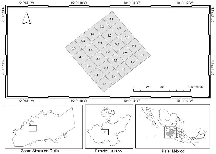
Figure 1 Study area and sampling plot location. The subplot arrangement is composed of the subplot row number and the subplot column number (n,n).

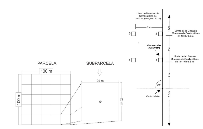
A 100 × 100 m forest sample plot was established in a representative area of Pinus-Quercus forest, with a 10 % slope and northwest orientation. The coordinates of its centroid are 20°17'51.89" north and -104°4'16.35" west. Its delimitation was carried out with topographic precision, using a Sokkisha TM10E theodolite with 5" accuracy. The orientation of the plot was determined with the slope. Starting from one of the corners, square subplots of 20 × 20 m were delimited to cover a total of 25 (Figure 2a); 30 × 30 cm microplots and a 15 m transect of total length were installed in each microplot as shown in Figure 2b (^{Rubio et al., 2016}).

Adapted from ^{Rubio et al. (2016)}.

Figure 2 a) Shape and distribution of the sampling plot and b) interior design of the nested subplots.

In the case of litter (L) and fermentation (F) fuel loads, the depths and percentages of coverages of these layers were measured in each microplot (Figure 2b ). The material was then collected in a plastic bag and transferred to the National Forest Fire Research Laboratory, located in the Experimental Station Altos de Jalisco (INIFAP), where it underwent a drying process in a semi-automatic oven (self-made) at 70 °C, until it reached a constant minimum moisture and weight (^{Xelhuantzi et al., 2011}). Once the dry weight values were obtained, the Organic Layer Load (OLL) was calculated, using an adaptation of the equations described by ^{Morfín et al. (2012)}.

In the nested transect of each subplot, the Fallen Woody Material (fWM) was counted using the planar intersection method described by ^{Brown et al. (1982)} and the classification by time delay 1, 10, 100 and 1 000 hours described by ^{Fosberg et al. (1970)} (Figure 2b). In the 1, 10 and 100-hour fuels, the diameter of each element was measured using a Pretul model 21454 vernier calibrator to obtain the Average Quadratic Diameters (AQD). Fuels with 1 000 hours were measured for diameter with a Truper^® model Fh-5m tape measure and their condition was identified as firm or rotten.

Estimates of unit area loading were made using the equations described by ^{Morfín et al. (2012)}. For practical purposes, fuel loads of 1, 10 and 100 hours were reclassified as Fine Woody Material (FWM), while those of 1 000 hours were reclassified as Coarse Woody Material (CWM), according to ^{Woodall and Monleon's criteria (2008)}. An exploratory data analysis was performed for each fuel component, based on its descriptive statistics. Likewise, at the subplot level, spatial analyses were carried out according to the equations described in Table 1 (^{Kalogirou, 2003}; ^{Pebesma, 2004}; ^{Townsend and Fuhlendorf, 2010}; ^{López, 2016}).

Table 1 Equations used for spatial analysis of fuel loads.

Equation	Variable
I=nW∑i=1n ∑j=1nwi,jzizj∑i=1nzi2	I = Moran´s index Moran's Index n = Number of observations W = Sum of weights wi,jz = Attribute deviation with characteristics xi
γ(h)= 12n(h)∑i=1nZxi-Z(xi+h)2	γh = Semivariance h= Distance interval Zxi = Sample value at a location xiZ(xi+h) = Value of the sample at interval distance h from xi
P=∑i=1nPi*Ai∑Ai	P = Thiessen Polygon Fuels Pi = Fuels measured in the subplot iAi= Area of influence of the subplot i
Z(X0)=∑i=1nλ*Z(xi)	Z(X0) = Inverse Weighted Distance Fuels (IWD) λ = Weight assigned to the sample
ZKO(X)=∑i=1nλ*Z(xi)	ZKO(X0) = Ordinary Kriging Fuels (OK)
RMSE=∑i=1n(y0-yi)n	RMSE = Root mean square error y0 = Predicted value yi = Observed value

The normality of the residuals of the interpolations was verified with the Shapiro-Wilk test. The interpolation method was chosen, since it presented the best RMSE adjustment. Correlation coefficients on the fuel components were estimated using the Spearman method. Statistical and geostatistical analyses were performed with the R Project gstat, lctools and rgdal libraries (^{Bivand et al., 2020}; ^{Kalogirou, 2020}; ^{Pebesma and Graeler, 2020}).

Results and Discussion

Fuel loads litter and fermentation

Table 2 shows the descriptive statistics for layers L and F. Layer L had average values of litter fuel load (L), litter layer depth (L_depth) and litter layer fuel bulk density (L_AD) of 17.95 Mg ha^-1, 4.68 cm and 4.07 g cm^-3 respectively. In layer F, the average values of fermentation fuel load (F), depth of the fermentation layer (F_depth) and bulk density of the fuel in the fermentation layer (F_AD) were 33.12 Mg ha^-1, 3.26 cm and 10.96 g cm^-3, respectively.

Table 2 Descriptive statistics for layers L and F.

Concept	Minimum	Quartile 1	Median	Mean	Quartile 2	Maximum	Unit
L	7.03	14.13	17.27	17.95	21.36	39.32	Mg ha^-1
L_depth	2.25	3.75	4.75	4.68	5.25	7.00	cm
L_AD	1.96	3.34	3.82	4.07	4.33	10.50	g cm^-3
F	4.37	18.58	27.59	33.12	49.16	100.59	Mg ha^-1
F_depth	0.33	1.75	2.50	3.26	4.25	9.25	cm
F_AD	7.03	9.40	10.93	10.96	11.78	17.97	g cm^-3

L = Litter layer; L_depth= Litter layer depth; L_AD= Litter layer fuel bulk density; F = Fermentation layer; F_depth = Depth of the fermentation layer; F_AD = bulk density of the fuel in the fermentation layer.

The fermentation layer presented a correlation coefficient of 0.96 p < 0.05, with respect to its depth; in the leaf litter layer it was 0.44 p < 0.05, with respect to its depth. Fuel loads were higher than those registered by ^{Bonilla et al. (2013)}, who cite values of 3.76 cm, 3.14 cm for depths, and 10.95 Mg ha^-1 and 9.00 Mg ha^-1 for L and F fuel loads, respectively. The L_AD and F_AD records were higher than those obtained by ^{Morfín et al. (2007)}, which were 1.67 and 6.79 g cm^-3 for L_AD and F_AD, respectively.

Fuel loads Fallen Woody Material

Descriptive statistics for the fWM fuels are summarized in Table 3. The root mean square diameters of the 1-, 10-, and 100-hour fuels were 0.23, 1.04, and 22.94 cm², respectively. Average values of 0.04, 0.49 and 2.7 Mg ha^-1 were obtained for the 1-, 10- and 100-hour fuels, while 0.22 and 0.34 Mg ha^-1 were obtained for the 1 000-hour firm (HF) and 1 000-hour rotten (HP) fuels, respectively. fWM fuels evidenced no apparent correlation, and their loads were lower than the ones documented by ^{Bonilla et al. (2013)}, whose values are 1.67, 0.62, 3.72 and 25.72 Mg ha^-1 for 1, 10, 100 and 1 000-hour fuels, respectively.

Table 3 Descriptive statistics for fWM fuels in Mg ha^-1.

Concept	Quartile 1	Median	Mean	Quartile 2	Maximum
1 H	0.00	0.00	0.04	0.08	0.39
10 H	0.00	0.35	0.49	1.05	1.74
100 H	0.00	0.00	2.70	3.56	14.23
1 000 HF	0.00	0.00	0.22	0.00	3.08
1 000 HP	0.00	0.00	0.34	0.00	4.09
FWM	0.35	1.74	3.23	3.91	14.58
CWM	0.00	0.00	0.57	0.00	4.24

fWM = Fallen Woody Material; FWM = Fine Woody Material; CWM = Coarse Woody Material.

Total and component fuel loads

Figure 3a shows the quantile distribution of the loadings grouped in F, L, FWM and CWM; Figure 3b shows the histogram of the total loadings. Together, the litter and fermentation layers concentrated 92.91 % of the total fuels, with an average of 54.86 ± 10.51 Mg ha^-1. The fermentation layer contributed the highest percentage, with 56.77 %, followed by the litter layer, with 36.14 %, while FWM and CWM together concentrated 7.09 % of the total fuels, with an average of 54.86 ± 10.51 Mg ha^-1. This means that, if fire is present in the area, the horizontal behavior will depend mainly on the litter and fermentation layers, with the existence of quite critical areas where fuel loads exceed 100 Mg ha^-1. The results are similar to those of ^{Rubio et al. (2016)}, authors who indicate an average load of 49.6 Mg ha^-1 for a stand with no fire, whose fermentation layer fuels are the most representative.

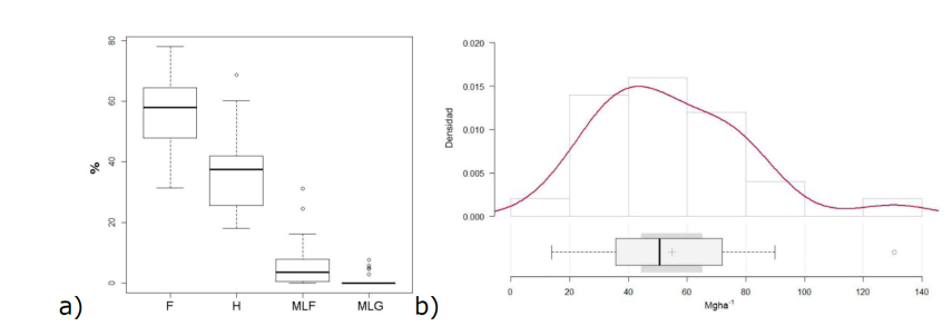
F = F; H = L; MLF =FWM; MLG = CWM; Densidad = Density.

Figure 3 a) Percentage contribution of the fuel components Fermentation (F), Litter (L), Fine Woody Material (FWM) and Coarse Woody Material (CWM) to total fuel loads; and b) Histogram of total fuel loads; the dark gray block represents the confidence interval of the mean.

Table 4 shows the fuel loads by component in the subplots, and Table 5 shows their correlation coefficients and p-values. The total fuel loads had a correlation coefficient of 0.97 with the fermentation component; this means that the fermentation fuel loads can be used as a basis for making inferences about the total loads. Furthermore, the correlation between the depth of the fermentation layer and its fuel load makes it possible to generate depth rates that allow for expeditious preliminary estimates.

Table 4 Fuel loads by component in the subplots (Mg ha^-1).

Subplot	Totals	F	L	FWM	CWM
1,1	53.11	27.59	17.52	3.91	4.09
1,2	71.86	49.23	21.59	1.05	0.00
1,3	58.32	32.92	21.84	3.56	0.00
1,4	75.29	49.16	25.01	1.12	0.00
1,5	33.68	19.54	14.13	0.00	0.00
2,1	46.90	21.10	19.63	3.71	2.45
2,2	65.39	26.07	39.32	0.00	0.00
2,3	13.92	4.37	9.56	0.00	0.00
2,4	70.17	42.72	27.10	0.35	0.00
2,5	31.11	13.84	17.27	0.00	0.00
3,1	38.85	18.58	7.03	12.10	1.14
3,2	40.06	25.72	14.33	0.00	0.00
3,3	54.01	33.69	15.71	4.60	0.00
3,4	89.83	53.89	21.36	14.58	0.00
3,5	29.04	10.02	11.91	7.11	0.00
4,1	35.77	15.51	16.70	3.56	0.00
4,2	79.38	51.10	17.19	11.10	0.00
4,3	72.59	49.32	18.60	0.43	4.24
4,4	30.06	17.21	12.86	0.00	0.00
4,5	50.57	27.89	19.12	3.56	0.00
5,1	130.53	100.59	24.91	5.03	0.00
5,2	81.91	63.99	16.87	1.05	0.00
5,3	45.71	26.15	17.67	1.90	0.00
5,4	48.16	32.38	11.82	1.74	2.21
5,5	25.27	15.35	9.57	0.35	0.00

F = Fermentation layer; L = Litter layer; FWM = Fine Woody Material; CWM = Coarse Woody Material.

Table 5 Correlation coefficients of the fuel components in the subplot.

Concept	Total	F	L	FWM	CWM
Totals	1	0.97	0.71	0.36	0.03
F	p < 0.05	1	0.59	0.35	0.03
H	p < 0.05	p < 0.05	1	0.06	-0.12
FMW	p = 0.07	p = 0.09	p = 0.76	1	0.22
CWM	p = 0.89	p = 0.89	p = 0.56	p = 0.28	1

F = Fermentation layer; L = Litter layer; FWM = Fine Woody Material; CWM = Coarse Woody Material.

Spatial dependence of fuel components

Figure 4 shows a set of correlograms of the fuel components F, L, FWM and CWM. All Moran indices were close to zero, with p-values > 0.05. This indicates that the fuel components are not spatially self-correlated.

F = F; H = L; MLF =FWM; MLG = CWM.

Figure 4 Correlograms of the fuel components F, L, FWM, and CWM.

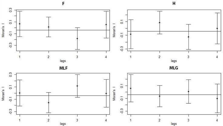
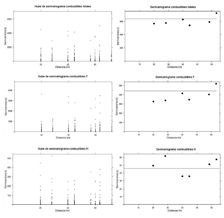
Figure 5 corresponds to the semivariograms and semivariogram clouds for the total F and L loads. The theoretical semivariograms with best fit to the experimental ones presented a complete seed behavior at 636.66, 439.55 and 45.00, with RMSE fit errors of 6.29, 8.99 and 0.82 for the total F and L loads, respectively. This confirms the randomness of the fuel loads shown by the spatial autocorrelation indices.

Distancia = Distance; Semivarianza= Semivariance; Semivariograma combustibles totales = Semivariogram total fuels; Nube de semivariograma combustibles = Semivariogram cloud fuels.

Figure 5 Semivariograms and semivariogram clouds for total F and L fuels.

Spatial interpolation of total fuels

Figure 6 shows the spatial distribution, in quantiles, of the residuals for the Thiessen, IWD and OK interpolations on the total fuel loads utilized for its estimation. The mean values of the residuals were 2.07, 0.04 and -0.001, with standard deviations of 34.08, 26.36 and 26.53 for Thiessen, IWD and OK, respectively. The lowest RMSE and variance of residuals were obtained in the IWD interpolation, with values of 25.82 and 694.60, followed by 25.98 and 703.46 for OK, and 33.46 and 1 161.87 for the Thiessen polygons. In all cases, the residuals exhibited a normal behavior with p-values of 0.40, 0.30 and 0.14 according to the Shapiro-Wilk normality test for Thiessen, IWD and OK, respectively. The spatial independence present in the fuel loads prevented the OK interpolation method from being superior to IWD. The RMSE values of IWD and OK were very similar; however, IWD recorded lower residual variances and, therefore, it was chosen as the interpolation method to be used.

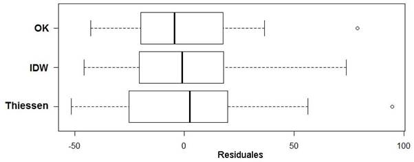
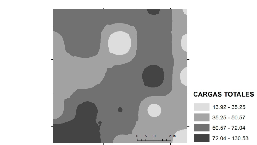
Figure 6 Residual distribution graphs.

Figure 7 shows the spatial distribution of total fuel loads in the sample plot. The percentage of the plot that exhibited fuel loads between 50.57 and 72.04 Mg ha^-1 was 48.28 %, while, 36.62 % had an interval of 35.25 to 50.57 Mg ha^-1. On the other hand, 10.70 % had the highest values of 72.04 to 130.53 Mg ha^-1, and only 5.65 % had the lowest values, of 13.92 to 35.25 Mg ha^-1. The spatial distribution of fuels showed the presence of areas with more than 100 Mg ha^-1, higher than the ones reported by ^{Morfín et al. (2007)}, whose loads are approximately 80 Mg ha^-1, in coniferous forests.

Figure 7 Spatial distribution of total fuel loads in the sample plot.

Compared to studies in which field data collection is based on sampling sites and clusters with radii generally smaller than 20 m, and whose results are extrapolated to a surface area of one hectare (^{Xelhuantzi et al., 2011}; ^{Conafor, 2011}; ^{Chávez et al., 2016}), measurements in the sampling plot allowed to identify variations in detail. The distance between the subplot with the smallest total load and the subplot with the largest total load is only 72.11 m, with a load difference of 116.61 Mg ha^-1. A sampling site with a radius of less than 20 m would hardly be able to represent such a difference in fuel loads. The results show the heterogeneity in the horizontal distribution of the dead fuel components in an area of one hectare. However, according to the methods described by ^{Velasco et al. (2013)}, the sampling plot should correspond to a homogeneous area.

Conclusions

In a one-hectare sample plot of Pinus-Quercus forest, dead forest fuel loads are spatially distributed independently, in a range of 13.92 to 130.53 Mg ha^-1, with no correlation between their components. This indicates that there are areas where fuel loads must be reduced in order to avoid further damage in the event of a forest fire. The sampling design utilized has identified detailed variations in fuel loads and evidences heterogeneity over a relatively small area. Measurements were made directly in the field, with a high level of detail; however, achieving the expected accuracy entails relating the availability of time to the economic resources. More sample plots are required in order to obtain replicates and analyze data between plots. The scaling of factors must be adjusted, based on further research, to create links between planning and operational activities. Interdisciplinary work and the development of integration methods must be encouraged in order to allow specialists from different areas to contribute their knowledge to achieve adequate fire management.

Acknowledgements

The authors are grateful to the Sierra de Quila Flora and Fauna Protection Area for its active participation and operational support in this work; to the Instituto Nacional de Investigaciones Forestales, Agrícolas y Pecuarias (Inifap) for the facilities granted to the authors; to Dr. Mariano García Alonso and Dr. María Inmaculada Aguado Suárez of the University of Alcalá, Spain, for their guidance and important contribution of knowledge; to Álvaro Pujol Becerra and PUJOL Ingeniería for their technical and operational support in the field work, and to the anonymous reviewers of this document for their valuable contribution.

REFERENCES

Bivand, R., T. Keitt, B. Rowlingson, E. Pebesma, M. Sumner, R. Hijmans, E. Rouault, F. Warmerdam, J. Ooms and C. Rundel. 2020. Package ‘rgdal’ 1.4-8. Bindings for the 'Geospatial' Data Abstraction Library. https://cran.r-project.org/web/packages/rgdal/rgdal.pdf (20 de junio de 2020). [ Links ]

Bonilla P., E., D. A. Rodríguez T., A. Borja D., C. Cíntora G. y J. Santillán P. 2013. Dinámica de combustibles en rodales de encino-pino de Chignahuapan, Puebla. Revista Mexicana de Ciencias Forestales 4(19): 21-33. Doi:10.29298/rmcf.v4i19.376. [ Links ]

Brown, J. K., R. D. Oberheu and C. M. Johnston. 1982. Handbook for inventoring surface fuels and biomass in the Interior West. USDA Forest Service, Intermountain Forest and Range Experiment Station, General Technical Report INT-129. Ogden, UT, USA, 48 p. [ Links ]

Chávez D., A. A., J. Xelhuantzi C., E. A. Rubio C., J. Villanueva D., H. E. Flores L. y C. De la Mora O. 2016. Caracterización de cargas de combustibles forestales: una herramienta importante para el manejo de los reservorios de carbono y su potencial contribución al cambio climático. Revista Mexicana de Ciencias Agrícolas. Vol. Esp.(13): 2589-2600. Doi: 10.29312/remexca.v0i13.485. [ Links ]

Comisión Nacional Forestal (Conafor). 2011. Manual y procedimientos para el muestreo de campo Re-muestreo inventario nacional forestal y de suelos (INFyS). Zapopan, Jal., México. 141 p. [ Links ]

Comisión Nacional Forestal (Conafor). 2020. Reporte semanal de resultados de incendios forestales, Coordinación General de Conservación y Restauración, Comisión Nacional Forestal, Gerencia de Manejo del Fuego. https://www.gob.mx/cms/uploads/attachment/file/604834/Cierre_de_la_Temporada_2020.PDF (30 de enero de 2021). [ Links ]

Flores G., J. G., D. A. Moreno G. y J. E. Morfín R. 2010. Muestreo directo y fotoseries en la evaluación de combustibles forestales. Folleto Técnico Núm. 4. INIFAP CIRPAC-Campo Experimental Centro Altos de Jalisco. Tepatitlán de Morelos, Jal., México. 69 p. [ Links ]

Fosberg, M. A., J. W. Lancaster and M. J. Schroeder. 1970. Fuel moisture response-drying relationships under standard and field conditions. Forest Science. 16(1): 121-128. Doi: 10.1093/forestscience/16.1.121. [ Links ]

Houtman, R. M., C. A. Montgomery, A. R. Gagnon, D. E. Calkin, T. G. Dietterich, S. McGregor and M. Crowley. 2013. Allowing a wildfire to burn: estimating the effect on future fire suppression costs. International Journal of Wildland Fire 22(7): 871-882. Doi: 10.1071/WF12157. [ Links ]

Kalogirou, S. 2003. The Statistical Analysis and Modelling of Internal Migration Flows within England and Wales. PhD Thesis School of Geography, Politics and Sociology. University of Newcastle upon Tyne. Newcastle upon Tyne, UK. 242 p. [ Links ]

Kalogirou, S. 2020. Package ‘lctools’ 0.2-8. Local Correlation, Spatial Inequalities, Geographically Weighted Regression and Other Tools. https://cran.r-project.org/web/packages/lctools/lctools.pdf (20 de junio de 2020). [ Links ]

Keane, R. E. 2015. Wildland Fuel Fundamentals and Applications. Springer International Publishing. New York, NY, USA. 195 p. [ Links ]

López V., C. 2016. A protocol for the ranking of interpolation algorithms based on confidence levels. International Journal of Remote Sensing 37(19): 4683-4697. Doi:10.1080/01431161.2016.1219461. [ Links ]

Morfín R., J. E., E. Alvarado C., E. J. Jardel P., R. E. Vihnanek R., D. K. Wright, J. M. Michel F., C. S. Wright , R. D. Ottmar, D. V. Sandberg y A. Nájera D. 2007. Fotoseries para la Cuantificación de Combustibles Forestales de México: Bosques Montanos Subtropicales de la Sierra Madre del Sur y Bosques Templados y Matorral Submontano del Norte de la Sierra Madre Oriental. Department of Agriculture, Forest Service, Pacific Northwest Research Station. Gen. Tech. Rep. PNW-GTR. Portland, OR, USA. 98 p. https://www.fs.fed.us/pnw/fera/publications/fulltext/PhotoSeriesMexicoUW-FERAPublication.pdf (20 de junio de 2020). [ Links ]

Morfín R., J. E. , E. J. Jardel P., E. Alvarado C. y J. M. Michel F. 2012. Caracterización y cuantificación de combustibles forestales. Comisión Nacional Forestal-Universidad de Guadalajara. Guadalajara, Jal., México. 59 p. http://queimadas.cptec.inpe.br/~rqueimadas/material3os/Evaluac_cuantific_de_combustibles_Forestales.pdf (9 de diciembre de 2019). [ Links ]

Pebesma, E. and B. Graeler. 2020. Package ‘gstat’ 2.0-6. Spatial and Spatio-Temporal Geostatistical Modelling, Prediction and Simulation. https://cran.r-project.org/web/packages/gstat/gstat.pdf (20 de junio de 2020). [ Links ]

Pebesma, E. J. 2004. Multivariable geostatistics in S: the gstat package. Computers & Geosciences, 30: 683-691. Doi: 10.1016/j.cageo.2004.03.012. [ Links ]

Pettinari, M. L. and E. Chuvieco S. 2016. Generation of a global fuel data set using the Fuel Characteristic Classification System. Biogeoscience 13: 2061-2076. Doi: 10.5194/bg-13-2061-2016. [ Links ]

Pyne, S. J., P. L. Andrews and R. D. Laven. 1996. Introduction to wildland fire. 2nd edition. John Wiley and Sons, Inc. New York, NY, USA. 769 p. [ Links ]

Rentería A., J. B. 2004. Desarrollo de modelos para el control de combustibles en el manejo de ecosistemas forestales en Durango, México. Tesis doctoral. Facultad de Ciencias Forestales. Universidad Autónoma de Nuevo León. Linares, NL., México. 141 p. [ Links ]

Riccardi, C. L., R. D. Ottmar, D. V. Sandberg, A. Andreu, E. Elman, K. Kopper and J. Long. 2007. The fuelbed: a key element of the Fuel Characteristic Classification System. Canadian Journal of Forest Research 37: 2394- 2412. Doi:10.1139/X07-143. [ Links ]

Rodríguez T., D. A., H. Tchikoué, C. Cíntora G., R. Contreras A. y A. De la Rosa V. 2011. Modelaje del peligro de incendio forestal en las zonas afectadas por el huracán Dean. Revista Agrociencia 45(5): 593-608. https://www.colpos.mx/agrocien/Bimestral/2011/jul-ago/art-6.pdf (20 de junio de 2020). [ Links ]

Rubio C., E. A., M. A. González T., J. D. Benavides S., A. A. Chávez D. y J. Xelhuantzi C. 2016. Relación entre necromasa, composición de especies leñosas y posibles implicaciones del cambio climático en bosques templados. Revista Mexicana de Ciencias Agrícolas Pub. Esp. (13): 2601-2614. Doi:10.29312/remexca.v0i13.486. [ Links ]

Secretaría del Medio Ambiente y Recursos Naturales (Semarnat) y Secretaría de Agricultura, Ganadería, Desarrollo Rural, Pesca y Alimentación (Sagarpa). 2007. NORMA OFICIAL MEXICANA NOM-015-SEMARNAT/SAGARPA-2007. Especificaciones técnicas de métodos de uso del fuego en los terrenos forestales y en los terrenos de uso agropecuario. Diario Oficial de la Federación. Ciudad de México, México. 32 p. http://www.dof.gob.mx/normasOficiales/3594/semarna/semarna.htm (20 de junio de 2020). [ Links ]

Sullivan, A. L. 2009. Wildland surface fire spread modelling, 1990-2007. 3: Simulation and mathematical analogue models. International Journal of Wildland Fire 18(4): 387-403. Doi: 10.1071/WF06144. [ Links ]

Townsend, D. E. and S. D. Fuhlendorf. 2010. Evaluating relationships between spatial heterogeneity and the biotic and abiotic environments. The American Midland Naturalist 163(2): 351-365. Doi:10.1674/0003-0031-163.2.351. [ Links ]

Velasco H., J. A., J. G. Flores G., B. Márquez A. y S. López. 2013. Áreas de respuesta homogénea para el muestreo de combustibles forestales. Revista Mexicana de Ciencias Forestales 4(15): 41-54. Doi: 10.29298/rmcf.v4i15.447. [ Links ]

Woodall, C. W. and V. J. Monleon. 2008. Sampling Protocol, Estimation, and Analysis Procedures for the Down Woody Materials Indicator of the FIA Program. United States Department of Agriculture. Forest Service Northern Research Station. General Technical Report NRS-22. Madison, WS, USA. 72 p. [ Links ]

Xelhuantzi C., J., J. G. Flores G. y A. A. Chávez D. 2011. Análisis comparativo de cargas de combustibles en ecosistemas forestales afectados por incendios. Revista Mexicana de Ciencias Forestales . 2(3): 37-52. Doi: 10.29298/rmcf.v2i3.624. [ Links ]

Received: May 29, 2020; Accepted: February 16, 2021

^{Conflict of interests}

The authors declare no conflict of interests.

^{Contribution by author}

Álvaro Agustín Chávez Durán: field data collection, laboratory sample processing, data analysis and drafting of the document; Abundio Bustos Santana: field data collection, data analysis and drafting of the paper; Héctor Manuel Chávez Durán: laboratory sample processing, data analysis and drafting of the document; Celia De la Mora Orozco: field data collection and drafting of the document; José Germán Flores Garnica: review of the document; Ernesto Alonso Rubio Camacho: review of the document; Jaqueline Xelhuantzi Carmona: review of the document.

Este es un artículo publicado en acceso abierto bajo una licencia Creative Commons