


Servicios Personalizados
Revista
Articulo
 texto en
  Inglés (pdf)
 Artículo en XML
 Referencias del artículo
 Enviar artículo por email
Indicadores
-
 Citado por SciELO
 -
 Accesos
Links relacionados
-
 Similares en
SciELO
Similares en
SciELO
Compartir

 Permalink
Revista mexicana de ciencias forestales
versión impresa ISSN 2007-1132
Rev. mex. de cienc. forestales vol.11 no.62 México nov./dic. 2020 Epub 19-Feb-2021
https://doi.org/10.29298/rmcf.v11i62.775
Scientific article
Comparative analysis of the number and intervals of forest fire risk classes
1Campo Experimental Centro Altos de Jalisco, Centro de Investigación Regional Pacífico Centro, INIFAP. México.
2Centro Universitario de Ciencias Biológicas y Agropecuarias. Universidad de Guadalajara. México
The issue of forest fires involves prioritizing areas of attention, based on criteria such as risk, in order to locate and size them on specific thematic maps. Their classification includes: a) selecting the number of risk classes, and b) a process to establish class intervals. However, this varies depending on the appreciation of who specifies such classification. In order to prevent this variation, a comparative analysis is made between two class numbers (3 and 5) and the following alternative categories: Equal Intervals, Quantiles, Natural Breaks, and Geometric intervals. 1 000 validation sites (VS) were located at random on a forest fire risk map of the state of Jalisco (Mexico) in order to determine the number of classes and the method for establishing the intervals. An area of 100 km2 was delimited around these sites, where the number of forest fires during the 2005-2014 period was determined. Thus, the risk class corresponding to each of these VS was associated with the number of fires that were located in the 100 km2 area. Based on this, the variability (standard deviation) between the classes generated by each of the four methods for determining their intervals was compared. The results suggest that the Equal Interval method is the most suitable for defining the intervals of the fire risk class. As for the number of classes, there is a clear differentiation between the classes when five of these are utilized.
Keywords Quantile; equivalent interval; geometric intervals; equal intervals; progression intervals; natural breaks
La problemática de incendios forestales conlleva a priorizar áreas de atención con base en criterios como el riesgo, para ubicarlas y dimensionarlas en cartografía temática específica; cuya clasificación implica: a) selección del número de clases de riesgo; y b) proceso para establecer los intervalos de clases. No obstante, esto varía dependiendo de la apreciación de quien especifica la clasificación; para evitarlo, se hace un análisis comparativo entre dos números de clases (3 y 5) y las siguientes alternativas de división de intervalos entre las clases: Intervalos iguales; Cuantiles; Rupturas naturales; e Intervalos geométricos. Se usó un mapa de riesgo de incendios forestales del estado de Jalisco (México), en el cual para definir el número de clases y el método para establecer los intervalos, se ubicaron al azar 1 000 sitios de validación (SV). Alrededor de ellos se delimitó una superficie de 100 km2, para contar el número de incendios forestales del período 2005-2014. Así, se asoció la clase de riesgo que correspondía a cada uno de los SV con el número de incendios ubicados en el área de 100 km2. A partir de esto, se comparó la variabilidad (desviación estándar) entre las clases generadas por cada uno de los cuatro métodos para definir sus intervalos. Los resultados sugieren que el método de intervalos iguales (II) es el más indicado para definir los intervalos de clase de riesgo de incendios. Referente al número de clases, existe una más clara diferenciación, entre las clases, al usar cinco clases.
Palabras clave Cuantil; intervalo equivalente; intervalo geométrico; intervalos iguales; intervalos de progresión; rupturas naturales
Introduction
In Mexico, fires impact forest ecosystems every year; for example, during the 2005-2015 period, an average of 8 857.9 fires occurred and affected 326 524.4 ha per year (Conafor, 2015). Jalisco, in particular, is one of the 10 states in which fires are most frequent, with an average of 595.9, affecting around 21 594 ha per year. This indicates that strategies to prevent and combat forest fires must be established (Calkin et al., 2014). However, because the available resources (both financial and human) are limited, it is necessary to prioritize the areas to be addressed (Conafor, 2010; Mildrexler et al., 2016), which can be located and sized using specific thematic maps (de la Riva et al., 2004).
These maps are generated according to several criteria, such as forest fire risk (Kuter et al., 2011; Mohammadi et al., 2014; Salvati and Ferrara, 2015) and hazard (Magaña and Romahn, 1987; Rojo et al., 2001). However, studies of fire risk in Mexico are scarce (Villers and López, 2004; Vega-Nieva et al., 2018), as the definition of criteria implies cartographically integrating a large amount of information (Carrillo et al., 2012), such as the occurrence of fires (Ávila et al., 2010; Pérez et al., 2013; Pan et al., 2016); nearness to roads (de Torres et al., 2008), slope, fuel loads, etc.
Sometimes, this integration requires complex processes (Vilar et al., 2011), and the resulting maps can have a limited use if not presented in a good way (Yeguez and Ablan, 2012); for which it is necessary to specify, among other aspects, the scale, orientation, georeferencing system, etc. through procedures that are well defined.
One of the aspects to which little attention has been given, besides the specification of the number of classes, in this case, of risk or danger of fire (Torres et al., 2007; Rodríguez et al., 2011), is the definition of the class intervals. Frequently, this is done randomly or from a subjective perspective, based on the personal appreciation of the creator of the maps. In principle, when generating a fire risk map, three (low, medium and high) or five (very low, low, medium, high and very high) risk classes are generally established. Traditionally, their intervals are then specified based on a division of the highest risk value by the number of classes, without any criteria to justify it.
There are several methods for defining the intervals of each class, including equal intervals, standard deviation, geometric interval, etc. (Osaragi, 2002); these are used indistinctly and, furthermore, are chosen subjectively. However, it is important to consider that comparing different risk classes, or class intervals, can result in considerable operational differences in relation to the location and dimensioning of those classes.
Accordingly, the objective of the present work was to make a comparative analysis between two classifications of the number of fires: three [low, medium and high] and five [very low, low, medium, high and very high]; the classes were defined according to different alternatives of interval division (equivalent interval, natural breaks, geometric interval and interval between quantiles). Based on this, an objective process is proposed to define the number of class intervals (of number of fires) in forest fire risk mapping. Thus, by using the same classification criteria, risk maps from different regions can be compared. The proposal is exemplified with georeferenced information on risk, which is defined in relation to the occurrence of forest fires in the state of Jalisco.
Number of forest fire risk classes. In practical terms, risk is defined as the probability of a forest fire starting (Flores, 2017) and is determined according to various criteria: closeness to roads, occurrence of fires, causes, etc. Each of these criteria is assigned a series of weightings that, when integrated, determine a certain value of forest fire risk in a particular place.
Subsequently, and due to budgetary constraints, priority areas of attention are established for which a number of specific risk classes are defined and maps representing their spatial distribution are generated. However, it is important to note that the specification of the number of risk classes depends on their illustrating in sufficient detail the spatial variation of forest fire risk. Therefore, a balance is sought between a very low number of classes, which does not allow for adequate detail of risk behavior in space, and a very high number that makes it difficult to locate and determine the size of each of the classes. This is generally defined based on perceptive aspects, as well as in relation to the experience of the person in charge of interpreting the information.
Thus, without any statistical support, three, four, five or more classes of forest fire risk are specified; for example: a) high, medium and low (Atienza et al., 2012; Sevillano et al., 2015); b) very high, high, moderate, low (Jaiswal et al., 2002); c) other extreme categories are added, such as zero risk and extreme risk (July, 1990), or very low and very high risk (IDEAM, 2011). In a similar way, for the definition of risk index maps, other risk determination indices can be adopted: a) Canadian: low, moderate, high, very high and extreme (Burriel et al., 2006); b) Australian: low, moderate, high, very high and extreme (Dowdy et al., 2009); c) American: low, moderate, high, very high and severe (Jolly et al., 2019); Brazilian: null, small, medium, high and very high (Ziccardi et al., 2020).
Specifying class intervals. Once the number of risk classes has been determined, the criteria for establishing the intervals for each of them must be defined. Although specific processes are followed, the intervals are selected in various ways, which implies that one can have different classification intervals for the same area. The classification of these processes is feasible with a mathematical or statistical perspective (Robinson, 1975), but they are generally determined under empirical criteria (Evans, 1977). In turn, these are subdivided into exogenous criteria and those determined from their spatial distribution (Evans, 1977). However, the approach tends rather to be arbitrary, with easily identifiable limits, disregarding the original distribution of the data (Evans, 1977).
In general, processes of a practical nature are used, for example: 1) to mathematically divide the interval of risk values by the number of classes to be established (Conafor, 2010; Castillo et al., 2012); 2) defining the frequency distribution of the risk values, so that the area corresponding to the first priority class is equal to half of the area of the second priority class, and this, to half of the third class (1/7, 2/7 and 4/7 of the total, respectively) (July, 1990); and 3) from the amplitude of the generated risk values, followed by the implementation of the following equation (IDEAM, 2011):
Where:
Min1 = Minimum normalized factor value across the study area
Max1 = Maximum normalized value presented by the factor in the whole study area
N = Total number of data for each factor
It should be noted that in no case is a statistical support used for the definition of the risk class interval.
Standard Classification Schemes. When establishing the class intervals with which the information will be classified on the fire risk map, first the spatial distribution of the data must be examined, because the following situations may occur (Osaragi, 2002): a) omission of the nature of the data; b) loss of data, when numerical values are classified and represented on maps for visual understanding; and c) as a consequence of the previous points, it is possible to misinterpret reality. Furthermore, the spread of imprecision generated by the processes of mapping with different classes must be considered (Goodchild et al., 1992). In addition, specification of the best arrangement of values among the different classes is sought; in general, two conditions are intended (Jenks and Coulson, 1963; Jenks 1967): a) the values within the classes must define the least variability; and b) the greatest variability among the considered classes must be achieved. According to the above, the following classification schemes are available:
Equivalent or equal intervals. A method that divides the range of attribute values into a sub-range of the same size (Olaya, 2014); recommended when the range of data is known, for example: percentages or temperature data. It can be used if one wishes to emphasize the quantity of a particular value in regard to the other values (Osaragi, 2002). However, it has the disadvantage of including an uneven number of elements within each class (some with many and others with few). This is relevant, since there can be elements with outliers that distort the meaning of the maximum and minimum, when defining the width of each class (Olaya, 2014).
Natural breaks. This method is based on Jenks' natural breakup algorithm (Jenks, 1967), in which breakpoints or group patterns are identified based on the data. The separation of the classification is divided into classes, whose boundaries are set where there are relatively large leaps in the values (Osaragi, 2002). In this way, it is intended to establish classes as homogeneous as possible through the reduction of variance within each one, thus defining classes that are well differentiated from one other (Olaya, 2014).
Geometric interval or progression intervals. A tool specifically designed to accommodate continuous data, with which classes are determined by creating breaks in the class intervals that have a geometric series. To optimize them, this coefficient can be changed once to its inverse; thus, the algorithm generates geometric intervals by minimizing the sum of squares of the number of elements in each class and ensuring that each class interval has approximately the same number of values and that the change between intervals is consistent (Olaya, 2014).
Intervals by quantiles. Based on a database, the median is divided into two equal parts, or more, called quantiles (quartiles, quintiles, deciles, and percentiles). Thus, all classes contain the same number of elements. For example, when defining quartiles, the database will be divided into four classes―each with an equal number of elements―, whose boundaries are located at the 25th, 50th, and 75th percentiles. The method is applicable when values are distributed on a linear basis (Osaragi, 2002).
Materials and Methods
Study area
The present work was developed by using information from the state of Jalisco, which is located in the central-western part of Mexico, on a surface area of 78 588 km2, of which 68 % has a warm sub-humid climate along the coast and in the central zone, while 18 % is temperate sub-humid in the upper parts of the mountains and 14 % is dry and semi-dry in the north and northeast. At a national scope, the entity occupies the tenth place by the number of registered forest fires, and the fourth place in terms of affected surface. On average, about 22 000 ha are burned each year (Figure 1), which corresponds to 570 fires per year, with an average of 30 ha per fire. The most damaged vegetation type is grassland, with an average of almost 12 000 ha per year; it is followed by forest areas with shrubs and bushes, with about 8 500 ha per year; and the burned area with the presence of adult trees amounts, on average, to 1 100 ha (Conafor, 2015).
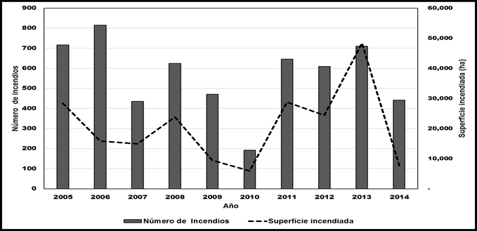
Source: Conafor (2015).
Número de incendios = Number of forest fires; Superficie incendiada = Area affected.
Figure 1 Number of forest fires and area affected during the 2005-2014 period in the state of Jalisco, Mexico.
Establishing the risk of fire
Factors such as topography, agricultural activities, fuel models, fire history, etc. are analyzed in order to locate and size the priority areas for forest fire fighting (Vilchis et al., 2015). Based on these, a map of priority attention areas is developed, indicating on it the pertinent preventive actions, under the corresponding management plan (Calkin et al., 2014).
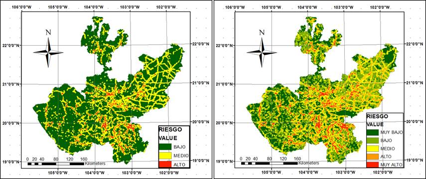
In Mexico, these areas are located and sized according to the determination of risk, hazard and value criteria (Conafor, 2010). Specifically, the concept of risk, in practical terms, refers to the probability of a forest fire occurring in a given area and within a given period (Hardy, 2005); this depends on various factors (Julio, 1990; Conafor, 2010; Rodríguez et al., 2011), which in turn are divided into a series of variables that receive a certain weighting (Table 1). Based on these, the spatial variation of risk assessments in the state of Jalisco was determined (Figure 2).
Table 1 Weighting criteria to determine the risk of forest fires.
| Factor | Variable | Criterion | Weighting |
|---|---|---|---|
| Locations | Proximity | 0 - 500 m | 4 |
| 500 - 1 000 m | 3 | ||
| 1 000 - 1 500 m | 2 | ||
| 1 500 - 2 000 m | 1 | ||
| Density | > 50 000 inhabitants | 2 | |
| < 50 000 inhabitants | 1 | ||
| Roads | Proximity | 0 - 500 m | 4 |
| 500 - 1 000 m | 3 | ||
| 1 000 - 1 500 m | 2 | ||
| 1 500 - 2 000 m | 1 | ||
| Type | Dirt road | 2 | |
| Paving | 1 | ||
| Historical ocurrence of fires |
Proximity | 0 - 500 m | 3 |
| 500 - 1 000 m | 2 | ||
| 1 000 - 2 000 m | 1 | ||
| Causes | Agricultural activities, smokers, bonfires | 4 | |
| Forestry activities, hunters, cleaning of roads, unknown | 3 | ||
| Other productive activities, burning in landfills, litigation, electrical discharges | 2 | ||
| Exploitations, railroad, others | 1 |
Source: Conafor (2010).
Number and range of classes
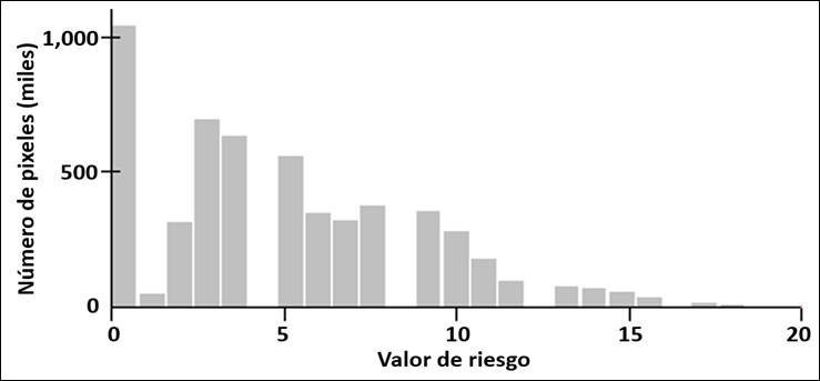
The forest fire risk map (Figure 2) was defined at the state level; thus, it was structured from a resolution of 120 × 120 m pixels, each of which was assigned a risk value. Figure 3 shows the frequency of these values, whose distribution tends to be normal, with an average of 5.102 and a variance of 3.929. While most of the pixels with risk are located between values 3 and 10, besides that there were few pixels with high values for risk. Based on this distribution, three and five classes were defined, being the most widely used (IDEAM, 2011; Atienza et al., 2012; Sevillano et al., 2015), whose intervals were defined with the following methods: a) Equal intervals (II); b) Quantities (Q); c) Natural breaks (QN); and d) Geometric intervals (IG). Subsequently, a comparative analysis (ANOVA) was made between methods, for each defined class.
Selection criteria
In order to define the number of classes and the most appropriate method to establish the corresponding intervals, 1 000 validation sites (SV) were first located at random throughout the state of Jalisco. Around each one, an area of 100 km2 was located (Figure 4), corresponding to the so-called fire risk factor (Flores, 2017; Flores and Macías, 2018), within which the total number of forest fires that occurred in the 2005-2014 period was counted. Thus, a class per site (SV) was associated with the number of fires counted in the 100 km2 area of each SV.
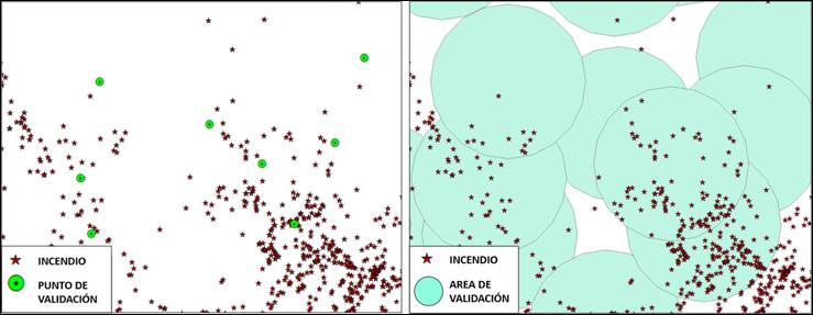
Incendio = Fire; Punto de validación = Validation sites (points); Área de validación = Validation area.
Figure 4 Detail of the location of the validation sites (points) and their corresponding area of 100 km2, within the state of Jalisco.
According to the method used to define the class intervals (three and five), each of the SV was identified with a risk class, which may differ according to the classification method. Based on the values of the number of fires in each one of the SV belonging to a risk class, the standard deviation was estimated as a parameter for comparison between the different classification methods. Finally, the thematic maps were elaborated, with the purpose of making a visual qualitative comparison displaying the differences and similarities between the tested classification methods.
Results and Discussion
Figure 5 shows the maps generated with the various classification methods; in general, there are similarities between the maps resulting from some of these. However, the spatial distribution of risk classes obtained with the equal interval method (II) is clearly different. This figure also shows the location of the boundaries of each interval, as determined by the utilized method.
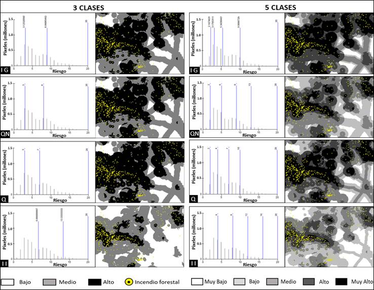
IG = Geometric Intervals; QN = Natural breaks; Q = Quantiles; II = Equal intervals.
Figure 5 Detail of the forest fire risk classification maps generated using different methods and number of classes.
Visual interpretation of risk classes
The analysis of the maps corresponding to three fire risk classes showed that there is no difference between the maps generated with the IG, QN and Q methods; besides, both the definition of the intervals' limits and their spatial distribution on the maps were very similar. However, the difference between method II with the IG, QN and Q methods is clear, since the High-risk class area was reduced, having been was absorbed mainly by the Medium-risk class. This can be seen in the graphic distribution of the limits of each one of the classes.
On the other hand, the maps that resulted from considering five classes were visually very different, which was also observed in the graphs corresponding to the limits of their intervals. However, it was clear the similarity between the maps derived from the GI and Q methods, in which the High and Very High risk classes covered a larger area. As in the case of the three classes, the map generated with thee II method had the largest difference. Although the differentiation between the five classes is evident, visually it is not recommended to use a very large number of classes, as complications may arise in the interpretation of the map when trying to identify the symbology of each class, potentially leading to errors (Olaya, 2014).
Fires by risk class
In order to characterize each of the risk classes, the number of forest fires present was evaluated (Table 2). When considering the classification of only three classes, the number of fires observed in class 1 (low risk) was the same, except when using method II, which exhibited over twice the number, compared to the other methods. As for class 2 (Medium risk), the behavior was similar, unlike the results obtained with the Q method, with registered only 84.5 % of the fires located using the IG and QN methods. Conversely, in class 3 (high risk) 6.54 % more fires were obtained using the Q method than with the IG and QN methods, while the II method exhibited only 43.3 % of fires, compared to IG and QN.
Table 2 Variation in total number of fires (A), average hectares per fire (B) and number of validation sites (C), by class and interval definition method.
| Class | 3-IG | 3-QN | 3-Q | 3-II | 5-IG | 5-QN | 5-II | 5-Q | |
|---|---|---|---|---|---|---|---|---|---|
| 1 | A | 429 | 429 | 429 | 952 | 296 | 296 | 540 | 296 |
| B | 7.00 | 7.00 | 7.00 | 5.48 | 6.79 | 6.79 | 7.24 | 6.79 | |
| C | 378 | 378 | 378 | 677 | 256 | 256 | 505 | 256 | |
| 2 | A | 1317 | 1317 | 1116 | 2535 | 133 | 442 | 1206 | 244 |
| B | 2.43 | 2.43 | 2.39 | 0.94 | 7.46 | 6.12 | 1.90 | 7.79 | |
| C | 424 | 424 | 355 | 294 | 122 | 349 | 297 | 249 | |
| 3 | A | 3071 | 3071 | 3272 | 1330 | 309 | 1359 | 1450 | 1005 |
| B | 0.54 | 0.54 | 0.67 | 0.20 | 5.53 | 1.47 | 0.89 | 1.75 | |
| C | 197 | 197 | 266 | 28 | 227 | 246 | 149 | 228 | |
| 4 | A | 1359 | 1390 | 1282 | 993 | ||||
| B | 1.47 | 0.64 | 0.26 | 1.45 | |||||
| C | 246 | 120 | 46 | 183 | |||||
| 5 | A | 2720 | 1330 | 339 | 2279 | ||||
| B | 0.42 | 0.20 | 0.09 | 0.33 | |||||
| C | 148 | 28 | 2 | 83 |
IG = Geometric Intervals; QN = Natural breaks; Q = Quantiles; II = Equal intervals.
In the five-interval classification, the II method exhibited 82.4 % more fires than the other methods. For class 2, there was variation in all cases, with a difference of 390.3 % between the lowest (IG) and the highest (II) number of fires. Classes 3 and 4 were more similar as to number of fires, while for class 5, the IG and Q methods yielded very similar numbers, although the QN and II methods exhibited 48.89 and 12.46 %, respectively, of the maximum number registered for IG class, which was 2 720 fires.
The average surface area per fire was very similar between methods when comparing the classes in the three-interval classification, although the Q and II methods presented lower values. As for the five-interval classification, in general, there was no definite trend, but the lowest values were obtained with the II method for all classes, except for class 1. The highest values varied by method in each of the five classes.
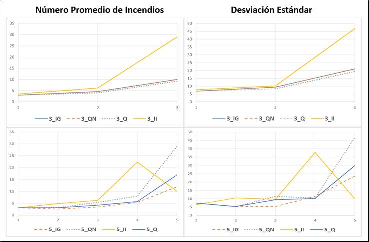
Variability between risk classes
Given that the definition of risk classes seeks the existence of sufficient variability among classes, Figure 6 shows that when only three classes were used, the variability (standard deviation) was practically the same among the classes defined with the IG, QN, and Q methods. However, when considering all the methods, there was a slight increase in variability in classes 1 and 2. Class 3 (high risk) is widely differentiated in the case of the II method; this agrees with the visual interpretation of the maps (Figure 5), in which the difference in the distribution and amplitude of the classes resulting from the application of method II was clear. On the other hand, when the average number of fires (Figure 6) corresponding to each class was considered, the observed behavior was very similar.
IG = Geometric Intervals; QN = Natural breaks; Q = Quantiles; II = Equal intervals.
Número promedio de incendios = Average number of fires; Desviación Estándar = Standard deviation.
Figure 6 Variation of the average number of fires and standard deviation, for each one of the forest fire risk classes.
When five classes were considered (Figure 6), the variability among the four methods was virtually the same. However, for risk class 2, the II method determined a greater standard deviation, while the other methods exhibited a similar variability. A better differentiation in the variability between the four methods was observed from class 3 (medium risk) onward.
In class 4 (high risk), the variability resulting from the II method stood out, while with the rest of the methods the variability was very similar and much lower. Finally, class 5 (very high risk) exhibited a clear difference between the variability of all the methods. As in the case of the three classes described above, the II method generated the best differentiation in the variability among its classes, followed by QN. On the other hand, in relation to the average number of fires per class, a slight variation was observed between the first three classes, considering all methods. This trend was also present in class 4, but only with the IG, QN and Q methods, as the II method exhibited a larger number of fires. In class 5, a clearer difference was registered between the number of fires when comparing the four methods.
These results suggest using, first, five class intervals instead of three. The equal interval (II) method was the best for defining the boundaries between classes. Accordingly, the number of classes must: a) not be so small that it will summarize the information excessively; b) allow for adequate detail of the spatial variation of the variable under study, and c) not be too large, so as to prevent the problems that ensued from not dividing the values into classes. In general, it is suggested not to use more than eight classes (Olaya, 2014).
As noted above, one of the purposes in selecting the interval of each of the classes is to ensure a statistically significant difference; thus, the ANOVAS (Table 3) resulting from the comparison of each of the classes supported the results of the analysis shown in Figure 6. For example, with the three-interval classification, no difference was observed in class 1 between the methods used, as confirmed by the resulting probability (p= 0.4430911), which implied the inexistence of a statistically significant difference, while a significant difference between the methods was registered in classes 2 and 3.
Table 3 ANOVA results comparing each of the defined classes using the different interval delimitation methods.
| Number of classes |
Class | F | Probability | Critical value of F |
|---|---|---|---|---|
| 3 | 1 | 0.89481466 | 0.443091101 | 2.609832328 |
| 3 | 2 | 3.18112253 | 0.023160437 | 2.61087455 |
| 3 | 3 | 6.90044144 | 0.000139627 | 2.617925093 |
| 5 | 1 | 0.00021454 | 0.999995655 | 2.61193174 |
| 5 | 2 | 4.73216689 | 0.0027658 | 2.613689205 |
| 5 | 3 | 3.3029531 | 0.019820786 | 2.615426601 |
| 5 | 4 | 18.0573828 | 3.18473E-11 | 2.619980452 |
| 5 | 5 | 2.85170654 | 0.037876469 | 2.63972568 |
On the other hand, in the five-interval classification, classes 2 to 5 exhibited a statistically significant difference when comparing between the methods.
Finally, it must be highlighted that this kind of work has not been done recently; therefore, no comparative analysis of the results obtained could be performed. This implies that since Jenks' study (1967), there has been little research on the definition of an analytical process for the selection of the number of classes and the most appropriate method for the delimitation of the intervals of those classes, such as might lead to an adequate classification of forest fire risk. The above research will provide statistical bases for a better location and sizing of the forest fire risk classes.
Conclusions
The results suggest that the equal interval method (II) is the most suitable one for defining the fire risk class intervals. Since, in the case of using three classes, although there are no differences in classes 1 and 2, there is clearly a greater variability in class 3. The variability observed by class with the rest of the methods is practically the same. When using five class intervals, the II method exhibits a different variability in classes 2, 4, and 5. In this case, an alternative method is the GI method, as it exhibits a differentiation in its variability in classes 3 and 5.
Regarding the number of classes, the results suggest that there is a greater differentiation between the classes when five class intervals are used; furthermore, this is observed in classes 2 to 5 and is more evident in class 5, in which all the methods exhibit a different variability as to the number of fires.
Based on the definition of forest fire risk, as shown by the results, a greater number is expected in the higher risk classes, although there was notably little variation in the first three risk categories.
It is important to emphasize that the results obtained in this work cannot be standardized for all the situations included in the definition of forest fire risk. However, the methodological process presented here is applicable in future research for determining both the number of risk classes and the limits of each class interval, and, therefore, preventing the use of subjective classifications. Furthermore, we suggest trying it with variations in intensities and in the shapes of validation sites, as well as with different numbers of classes.
Referencias
Atienza H., J., P. Muñoz A. y P. Balladares S. 2012. Determinación de prioridades de protección contra incendios forestales en la región de Valparaíso, Chile. Revista Cartográfica (88):147-82. https://www.researchgate.net/profile/Pedro_Munoz11/publication/327557748_Determinacion_de_Prioridades_de_Proteccion_Contra_Incendios_Forestales_en_la_Region_de_Valparaiso_Chile/links/5b9667d5a6fdccfd543a0e84/Determinacion-de-Prioridades-de-Proteccion-Contra-Incendios-Forestales-en-la-Region-de-Valparaiso-Chile.pdf#page=149 (12 de mayo de 2020). [ Links ]
Ávila F., D. Y., M. Pompa G. y E. Vargas P. 2010. Análisis espacial de la ocurrencia de incendios forestales en el estado de Durango. Revista Chapingo. Serie Ciencias Forestales y del Ambiente 16 (2):253-260. Doi: 10.5154/r.rchscfa.2009.08.028. [ Links ]
Burriel M., J. A., F. X. Castro D., T. Mata B., D. Montserrat A., E. Gabriel de F. y J. J. Ibáñez I. M. 2006. La mejora del mapa diario de riesgo de incendio forestal en Cataluña. In: XII Congreso Nacional de Tecnologías de la Información Geográfica. Granada. 20 de septiembre de 2006. Editorial Universidad de Granada. Santa Perpetua de Moguda, España. pp. 651-666. [ Links ]
Calkin, D. E., J. D. Cohen, M. A. Finney and M. P. Thompson. 2014. How risk management can prevent future wildfire disasters in the wildland-urban interface. PINAS 111 (2):746-751. Doi:10.1073/pinas.1315088111. [ Links ]
Carrillo G., R. L., D. A. Rodríguez T., H. Tchikoué, A. I. Monterroso R. y J. Santillán P. 2012. Análisis espacial de peligro de incendios forestales en Puebla, México. INTERCIENCIA 37 (9):678-683. https://www.redalyc.org/pdf/339/33925502012.pdf (29 mayo de 2020). [ Links ]
Castillo S., M., R. Garfias S., G. Julio A. y L. González R. 2012. Análisis de grandes incendios forestales en la vegetación nativa de Chile. INTERCIENCIA 37 (11):796-804. https://www.redalyc.org/pdf/339/33925550002.pdf (29 de mayo de 2020). [ Links ]
Comisión Nacional Forestal (Conafor). 2010. Procedimiento para elaboración de un mapa de áreas de atención prioritaria contra incendios forestales. Comisión Nacional Forestal. Zapopan, Jal., México. pp. 9-11. [ Links ]
Comisión Nacional Forestal (Conafor). 2015. Reportes semanales de resultados de incendios forestales. Información de cierre de estadísticas de incendios forestales del 2007 al 2015. Comisión Nacional Forestal. Coordinación de Conservación y Restauración. Gerencia de Protección Contra Incendios Forestales. México, D.F., México. https://snigf.cnf.gob.mx/incendios-forestales/ (29 de mayo de 2020). [ Links ]
de la Riva, J., F. Pérez-Cabello, N. Lana-Renault and N. Koutsias. 2004. Mapping wildfire occurrence at regional scale. Remote Sensing of Environment (92):288-294. Doi:10.1016/j.rse.2004.06.013. [ Links ]
de Torres, C. M., L. Ghermandi y G. Pfister. 2008. Los incendios en el noroeste de la Patagonia: su relación con las condiciones meteorológicas y la presión antrópica a lo largo de 20 años. Ecología Austral 18 (2):153-167. http://www.scielo.org.ar/scielo.php?script=sci_arttext&pid=S1667-782X2008000200001 (12 de febrero de 2020). [ Links ]
Dowdy, A. J., G. A. Mills, K. Finkele and W. de Groot. 2009. Australian fire weather as represented by the McArthur Forest Fire Danger Index and the Canadian Forest Fire Weather Index. The Centre for Australian Weather and Climate Research. Melbourne, Australia. 84 p. [ Links ]
Evans, I. 1977. The selection of class intervals. Institute of British Geographers, Transactions (New Series) 2 (1):98-124. https://scihub.wikicn.top/10.2307/1791177 (12 de febrero de 2020). [ Links ]
Flores G., J. G. 2017. Unidad de muestreo para determinar la variabilidad espacial de la superficie quemada por incendios forestales. Revista Mexicana de Ciencias Forestales 8 (43):117-142. Doi:10.29298/rmcf.v8i43.68. [ Links ]
Flores G., J. G. and A. Macías M. 2018. Bandwidth selection for kernel density estimation of forest fires. Revista Chapingo Serie Ciencias Forestales y del Ambiente 24 (3):313-327. Doi: 10.5154/r.rchscfa.2017.12.074. [ Links ]
Goodchild, M. F., S. Guoqing and Y. Shiren 1992. Development and test of error model for categorical data. International Journal of Geographical Information Systems 6 (2):87-104. Doi:10.1080/02693799208901898. [ Links ]
Hardy, C. C. 2005. Wildland fire hazard and risk: Problems, definitions, and context. Forest Ecology and Management (211):73-82. Doi:10.1016/j.foreco.2005.01.029. [ Links ]
Instituto de Hidrología, Meteorología y Estudios Ambientales (IDEAM). 2011. Protocolo para la realización de mapas de zonificación de riesgos a incendios de la cobertura vegetal. Instituto de Hidrología, Meteorología y Estudios Ambientales Bogotá, D.C., Colombia. 109 p. [ Links ]
Jaiswal, R. K., S. Mukherjee, K. D. Raju and R. Saxena 2002. Forest fire risk zone mapping from satellite imagery and GIS. International journal of applied earth observation and geoinformation (4):1-10. Doi:10.1016/S0303-2434(02)00006-5. [ Links ]
Jenks, G. F. and M. Coulson. 1963. Class intervals for statistical maps. International Yearbook of Cartography 4 (3):119-134. https://www.semanticscholar.org/paper/Class-intervals-for-statistical-maps-Jenks-Coulson/28e9a6f1c5a56982147761c0a4a3cb6d5f2e4814 (18 de octubre de 2019). [ Links ]
Jenks, G.F. 1967. The data model concept in statistical mapping. International Yearbook of Cartography (7):186-190. Doi:10.1371/journal.pone.0061104. [ Links ]
Jolly, W. M., P. H. Freeborn, W. G. Page and B. W. Butler. 2019. Severe Fire Danger Index: A Forecastable Metric to Inform Firefighter and Community Wildfire Risk Management. Fire: 2(47): 2-24. Doi:10.3390/fire2030047. [ Links ]
Julio A., G. 1990. Diseño de índices de riesgo de incendios forestales para Chile. Bosque 11 (2):59-72. Doi: 10.4206/BOSQUE.1990.v11n2-06. [ Links ]
Kuter, N., F. Yenilmez and S. Kuter. 2011. Forest fire risk mapping by kernel density estimation. Croatian Journal of Forest Engineering 32 (2):599-609. http://www.crojfe.com/site/assets/files/3793/13kuter_599-610.pdf (4 de marzo de 2020). [ Links ]
Magaña T., S. O. y F. C. Romahn V. 1987. Determinación del índice de peligro de incendio forestal para Tlahuapan, Puebla. Ciencia Forestal 12: 58- 67. [ Links ]
Mildrexler, D., Z. Yang, W. B. Cohen and D. M. Bell. 2016. A forest vulnerability index based on drought and high temperatures. Remote Sensing of Environment (173):314-325. Doi: 10.1016/j.rse.2015.11.024. [ Links ]
Mohammadi, F., M. R. Bavaghar and N. Shabanian 2014. Forest fire risk zone modeling using logistic regression and GIS: an Iranian case study. Small-scale Forestry (13): 117-125. Doi: 10.1007/s11842-013-9244-4. [ Links ]
Olaya, V. 2014. Sistemas de información geográfica. CreateSpace Independent Publishing Platform. Madrid, España. 854 p. https://volaya.github.io/libro-sig/ (21 de abril de 2020). [ Links ]
Osaragi, T. 2002. Classification methods for spatial data representation. Center for advanced spatial analysis (CASA). University College London. London, United Kingdom. Working Paper Series No. 40. 19 p. [ Links ]
Pan, J., W. Wang and J. Li, 2016. Building probabilistic models of fire occurrence and fire risk zoning using logistic regression in Shanxi Province, China. Natural Hazards (81):1879-1899. Doi: 10.1007/s11069-016-2160-0. [ Links ]
Pérez V., L. Márquez, O. Cortés y M. Salmerón 2013. Análisis espacio-temporal de la ocurrencia de incendios forestales en Durango, México. Madera y Bosques 19(2):37-58. Doi:10.21829/myb.2013.192339. [ Links ]
Robinson, A. H. and B. B. Petchenik 1975. The Map as a communication system. Cartographic Journal (12):7-15. Doi: 10.1179/caj.1975.12.1.7. [ Links ]
Rodríguez, T., D. A., C. T Chikoué, C. Cíntora G., R. Contreras A. y A. de la Rosa V. 2011. Modelaje del peligro de incendio forestal en las zonas afectadas por el huracán Dean. Agrociencia 45 (5):593-608. http://www.scielo.org.mx/scielo.php?pid=S1405-31952011000500006&script=sci_arttext&tlng=pt (4 de marzo de 2020). [ Links ]
Rojo, M., P. Santillán, M. Ramírez y B. Arteaga M. 2001. Propuesta para determinar índices de peligro de incendio forestal en bosque de clima templado en México. Revista Chapingo, Serie Ciencias Forestales y del Ambiente 7 (1):39-48. [ Links ]
Salvati, L. and A. Ferrara 2015. Validation of MEDALUS Fire Risk Index using Forest Fire Statistics through a multivariate approach. Ecological Indicators 48:365-369. Doi:10.1016/j.ecolind.2014.08.027. [ Links ]
Sevillano, M. E., O. A. Toro y P. A. Ruiz 2015. Aplicación de SIG al análisis de riego pro incendios forestales en el municipio de Yotoco Colombia, 2014. 2015. In: Memorias de resúmenes en extenso SELPER-XXI-México-UACJ-2015. 12-16 de octubre de 2015. Ciudad Juárez, Chih., México. pp. 12-16. [ Links ]
Torres R., J. M., O. S. Magaña T. y. G. A. Ramírez F. 2007. Índice de peligro de incendios forestales de largo plazo. Agrociencia 41 (6):663-674. http://www.scielo.org.mx/pdf/agro/v41n6/1405-3195-agro-41-06-663-en.pdf (28 de mayo de 2020). [ Links ]
Vega-Nieva, D., J. Briseño-Reyes, M. Nava-Miranda, E. Calleros-Flores, P. López-Serrano, J. Corral-Rivas, E. Montiel-Antuna, M. I. Cruz-López, M. Cuahutle, R. Ressl, E. Alvarado-Celestino, A. González-Cabán, E. Jiménez, J. Álvarez-González, A. Ruiz-González, R. Burgan and H. Preisler. 2018. Developing Models to Predict the Number of Fire Hotspots from an Accumulated Fuel Dryness Index by Vegetation Type and Region in Mexico. Forests 9(4):190. Doi:10.3390/f9040190. [ Links ]
Vilar, H. L., M. P. Martín I. and F. J. Martínez V. 2011. Logistic regression models for human-caused wildfire risk estimation: analyzing the effect of the spatial accuracy in fire occurrence data. European Journal of Forest Research 130:983-996. Doi:10.1007/s10342-011-0488-2. [ Links ]
Vilchis, F., A. Y., C. Díaz D., D. Magaña L., K. M. Bá y M. A. Gómez A. 2015. Modelado espacial para peligro de incendios forestales con predicción diaria en la cuenca del río Balsas. Agrociencia 49 (7): 803-820. http://www.scielo.org.mx/scielo.php?pid=S1405-31952015000700008&script=sci_arttext&tlng=pt (18 de mayo de 2020). [ Links ]
Villers R., L. y J. López B. 2004. Comportamiento del fuego y evaluación del riesgo por incendios en las áreas forestales de México: un estudio en el Volcán la Malinche. In: Villers R., L. y J. López B . (eds.). Incendios forestales en México. Métodos de evaluación. Centro de Ciencias de la Atmósfera, UNAM. México, D.F., México. pp. 57-74. [ Links ]
Yeguez, M. y M. Ablan. 2012. Índice de riesgo de incendio forestal dinámico para la cuenca alta del río Chama. Revista Forestal Venezolana 56 (2):127-134. https://www.researchgate.net/profile/Magdiel_Ablan/publication/260427040_Indice_de_riesgo_de_incendio_forestal_dinamico_para_la_cuenca_alta_del_rio_Chama/links/004635313b5d7752a7000000/Indice-de-riesgo-de-incendio-forestal-dinamico-para-la-cuenca-alta-del-rio-Chama.pdf (16 de febrero de 2020). [ Links ]
Ziccardi, L., C. R. Thiersch, A. Miho Y. , P. Fearnside and P. J. Ferreira F. 2020. Forest-fire risk indices and zoning of hazardous areas in Sorocaba, São Paulo state, Brazil. Journal of Forestry Research 31(2): 581-590. Doi:10.1007/s11676-019-00889-x. [ Links ]
Received: May 25, 2020; Accepted: September 11, 2020
 Este es un artículo publicado en acceso abierto bajo una licencia
Creative Commons
Este es un artículo publicado en acceso abierto bajo una licencia
Creative Commons
