


Services on Demand
Journal
Article
 text in
  English (pdf)
 Article in xml format
 Article references
 Send this article by e-mail
Indicators
-
 Cited by SciELO
 -
 Access statistics
Related links
-
 Similars in
SciELO
Similars in
SciELO
Share

 Permalink
Revista mexicana de ciencias forestales
Print version ISSN 2007-1132
Rev. mex. de cienc. forestales vol.11 n.60 México Jul./Aug. 2020 Epub Dec 09, 2020
https://doi.org/10.29298/rmcf.v11i60.711
Scientific article
Diameter, height, basal area and volume growth of three pine species from Chihuahua, Mexico
1Instituto Tecnológico de El Salto. México.
The estimation of the growth and the yield of timber forest species is a decisive activity in the sustainable planning and projection of the forest harvest. The purpose of the present study was to adjust four regression models to estimate the diameter, basimetric area, height and volume growth of Pinus leiophylla, Pinus lumholtzii and Pinus strobiformis in Guadalupe y Calvo, Chihuahua, Mexico. Through selective sampling, 26 Pinus lumholtzii trees, 26 P. strobiformis trees, and 30 P. leiophylla trees were collected in order to generate 219, 249 and 385 profiles, respectively, of each of these species. The adjusted models utilized were those of Chapman-Richards, Schumacher, Hossfeld I and Weibull. The criteria for selecting the best-adjusted models were the coefficient of determination, the root mean square error, the significance of the estimated parameters, and the growth tendency curves. All the models were well adjusted; however, when the growth and yield projection curves were considered, the models that best represented the biological growth trend of the tree species were those of Chapman-Richards, Hossfeld I and Schumacher. Considering the age of maximum growth and the rotation age, the studied species exhibit a low growth.
Key words: Height; basimetric area growth; Pinus leiophylla Schiede ex Schltdl. & Cham.; Pinus lumholtzii B.L.Rob. & Fernand; Pinus strobiformis Engelm.; volumen growth
La estimación del crecimiento y rendimiento de las especies forestales maderables es clave para planear y proyectar la cosecha de manera sustentable. El objetivo de la presente investigación fue ajustar cuatro modelos de crecimiento en diámetro, altura, área basal y volumen para Pinus leiophylla, Pinus lumholtzii y Pinus strobiformis de la región de Guadalupe y Calvo, Chihuahua. Mediante un muestreo selectivo se recolectaron 26 árboles de P. lumholtzii, 26 de P. strobiformis y 30 árboles de P. leiophylla para generar 219, 249 y 385 perfiles de cada una de las especies, respectivamente. Los modelos de crecimiento evaluados fueron los de Chapman-Richards, Schumacher, Hossfeld I y Weibull. Los criterios de selección de los mejores modelos fueron el coeficiente de determinación, la raíz del error medio cuadrático, la significancia de los parámetros estimados y las tendencias del crecimiento. Se determinó que todos los modelos presentaron ajustes significativos; sin embargo, por las tendencias del crecimiento que generan, los que mejor representaron el comportamiento biológico de las variables analizadas fueron los de Chapman-Richards, Hossfeld I y Schumacher. Con base en las edades a las que ocurre el máximo incremento en volumen y el turno, se infiere que las tres especies presentan lento crecimiento.
Palabras clave: Altura; crecimiento en área basal; Pinus leiophylla Schiede ex Schltdl. & Cham.; Pinus lumholtzii B.L.Rob. & Fernand; Pinus strobiformis Engelm.; volumen
Introduction
Sustainable forest management must be supported by information that indicates the current conditions of tree growth and its subsequent development dynamics, in order to guarantee sustained production (Gyawali et al., 2015). This reference is essential to inform and support decision making regarding the management practices to be applied (López and Tamarit, 2005). In order to anticipate the response of the forest to forestry practices and estimate the volume generated over time, it is necessary to generate and apply equations that will allow predicting tree growth based on the age. These require significantly reliable levels of precision (Monárrez and Ramírez, 2003; Quiñonez et al., 2015; González et al., 2016) in order to guarantee a good definition of the most appropriate timber volume and age of a tree for commercial exploitation (Valdéz and Lynch, 2000). Within this context, growth estimation is a key factor in planning and predicting sustainable harvesting and implementing better silvicultural alternatives (Salazar et al., 1999; Corral and Návar, 2005), as well as updating forest inventory information (Imaña and Encinas, 2008; Quiñonez et al., 2015).
Depending on the type of forest, regular or irregular to be managed or assess, the study of growth can be approached at the stand level, by diameter classes or by individual trees (Piennar and Rheney, 1995; Gizachew and Brunner 2011). Growth models of individual trees have commonly been generated through stem analyses in order to describe the growth dynamics of timber species that occur in irregular forest areas (Torres and Magaña, 2001). Therefore, in many cases, avoiding periodic remediation facilitates the estimation and analysis of growth dynamics. In turn, the sum of the growth of individual trees results in growth at the stand level (Diéguez et al., 2009).
Studies on the construction of individual tree growth models for species of the genus Pinus with commercial timber importance in the state of Chihuahua are limited. For this reason, the objective was set to adjust and evaluate models that allow the estimation of growth and increases in diameter, basimetric area, height and volume for Pinus leiophylla Schiede ex Schltdl. P. lumholtzii. B.L. Rob. & Fernand, P. strobiformis Engelm. in the Guadalupe y Calvo region, Chihuahua.
Materials and Methods
Study area
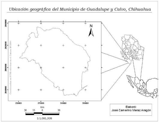
The study was conducted in the Forest Management Unit 0808 in Guadalupe y Calvo, Chihuahua (Figure 1), whose area covered by species of the Pinus and Quercus genera is 642 551 ha (Chávez et al., 2009), located north of the Western Sierra Madre and the south of the state of Chihuahua, within the R10, the Sinaloa Watershed. The predominant climate according to Köppen’s classification modified by García (2004) is temperate semi-cold and sub-humid, with a rainy, cool summer C(e)(w2)(x’). The soils exhibit an albic B subsurface horizon with a medium to thick texture and moderate organic matter content; these soils are classified as Pheozem, Cambisol, Regosol, Litosol, Planosol and Acrisol. The mosaic of temperate plant communities is formed by pure coniferous forests and mixed coniferous and broadleaf forests (Chávez et al., 2009).
Sampling
A sample of 26 P. lumholtzii and P. strobiformis trees, and 30 P. leiophylla trees was collected through targeted sampling in order to include three levels of seasonal quality (low, medium and high); the selected individuals were dominant and co-dominant and exhibited no physical damage. The minimum age for P. lumholtzii was 42 years; while those for P. strobiformis and P. leiophylla were 52 and 75 years, respectively. The selected trees allowed the reconstruction of 219 profiles of P. lumholtzii, 249 of P. strobiformis, and 385 of P. leiophylla, with the stem analysis technique (Klepac, 1983) for estimating the growth and annual increment in diameter, height, basimetric area and volume. Periods of ten years were considered for this purpose.
The reconstruction of the profiles was carried out by measuring and analyzing different diameters and recording the respective ages of the slices, which were obtained from each tree at a height of 0.30 m and 1.30 m from the ground, and then at every 2.60 m, up to the tip of the tree, in order to commercially exploit each of the logs that were extracted.
Variables
The variables of interest were species; normal diameter with bark; diameter without bark of each slice, measured with a Lufkin® rule, starting at the stump; the height of each section, and the number of rings of each slice. The annual growth rings were grouped into 10-year age classes in order to facilitate the estimation of the growth of the normal diameter and the basimetric area. The prediction of the true height per section of the slices was estimated using the formula by Carmean (1972) subsequently modified by Newberry (1991), as expressed in Equation 1.
Where:
hij = Estimated slice height of the i th slice, corresponding to growth ring j
h i = Accumulated height at the top cut of the i th slice
hi+1 = Accumulated height up to the upper cut of the previous i th slice
r i = Number of growth rings of each slice
j = Growth rings from the pith in each slice
The equations for cylinder (2), Smalian (3) and cone (4), respectively, were used to estimate the volume of each section per tree (i.e. of the stump, logs and tip of each tree).
Where:
Vi = Log volume
Dt = Upper diameter of the stump
DM = Largest diameter of each log
Dm = Smallest diameter of each log
Db = Diameter of the base of the tip (m)
l = Length of the log (m)
Statistical analysis
The quality of the statistical regression adjustment of four growth models was evaluated in order to estimate growth in diameter, basimetric area, height and bark-free volume (Table 1). The respective expressions of these models for the aim of estimating the current annual increment (CAI) and the mean annual increment (MAI) of individual trees (Kiviste et al., 2001) was also assessed, which are obtained by applying the first derivative to the growth function, and dividing the growth function by the age, respectively.
Table 1 Evaluated growth models and expressions for determining the CAI and MAI.
| Name | Models | CAI | MAI |
|---|---|---|---|
| Chapman-Richards |
|
|
|
| Hossfeld I |
|
|
|
| Schumacher |
|
|
|
| Weibull |
|
|
|
y = Growth in diameter (cm), basimetric area (m2), height (m) and volume (m3); t = Age (years); a b and c = Model parameters, CAI = Current annual increment in diameter (cm), basimetric area (m2), height (m), and volume (m3); MAI = Mean annual increment in diameter (cm), basimetric area (m2), height (m), and volume (m3).
The adjustment was made by applying the PROC MODEL procedure of the SAS statistical software (SAS, 2002). The goodness of fit of each model was determined by considering the adjusted coefficient of determination ( Adj R 2 ), the root mean square error (RMSE), and the significance of the parameters for selecting the most efficient model. Also, it was considered the graphic analysis of the growth trend curves, CAI and MAI.
The observed data of the growth of the analyzed variables kept a serial relationship through time, so that the observations are correlated. This causes the errors of the adjusted regression functions to be correlated as well. Therefore, the significance of this dependence was evaluated for each adjusted model by means of the Durbin-Watson autocorrelation test (d) (Sharma et al., 2011; Quiñonez et al., 2018), which is expressed as follows (5):
Where:
The autocorrelation between the errors of the best models was corrected by applying the auto-regression model CAR(X) developed by Zimmerman et al. (2001). This model allows to adjust the parameters of each of the growth models with those of the autoregressive model together. The structure of the autoregressive model is:
Where:
After selecting the best model for each analyzed species and variable, the maximum annual increase (CAI max ), the maximum annual increase (MAI max ) and the point of intersection CAI-MAI (node) were estimated.
Results
Growth models
Table 2 shows the statistics for the goodness-of-fit of the growth functions evaluated by species. Determination coefficients above 0.95 and standard errors below 2.4 cm for P. leiophylla and P. lumholtzii indicated a good fit for the four models tested for growth in diameter. For P. strobiformis, these same indicators suggested that only Chapman-Richards, Hossfeld I and Schumacher models had a good fit.
Table 2 Statistics of fit of growth models evaluated by variable and by species.
| Model | P. leiophylla | P. lumholtzii | P. strobiformis | |||
|---|---|---|---|---|---|---|
| Adj R 2 | RMSE | R 2 | RMSE | R 2 | RMSE | |
| Normal diameter | ||||||
| Chapman-Richards | 0.9852 | 1.2960 | 0.9594 | 2.1824 | 0.9666 | 1.9555 |
| Hossfeld I | 0.9807 | 1.4805 | 0.9508 | 2.4031 | 0.9628 | 2.0618 |
| Schumacher | 0.9840 | 1.3463 | 0.9570 | 2.2463 | 0.9643 | 2.0199 |
| Weibull | 0.9850 | 1.3069 | 0.9597 | 2.1742 | 0.8413 | 4.2602 |
| Basimetric area | ||||||
| Chapman-Richards | 0.9853 | 0.0041 | 0.9696 | 0.0057 | 0.9792 | 0.0051 |
| Hossfeld I | 0.9812 | 0.0046 | 0.9610 | 0.0065 | 0.9734 | 0.0058 |
| Schumacher | 0.9845 | 0.0042 | 0.9682 | 0.0059 | 0.9787 | 0.0052 |
| Weibull | 0.9848 | 0.0041 | 0.9696 | 0.0057 | 0.9794 | 0.0051 |
| Total height | ||||||
| Chapman-Richards | 0.9172 | 2.0734 | 0.9422 | 1.8089 | 0.9187 | 1.9792 |
| Hossfeld I | 0.9172 | 2.0710 | 0.9380 | 1.8717 | 0.8209 | 2.9365 |
| Schumacher | 0.9179 | 2.0613 | 0.9428 | 1.7992 | 0.9167 | 2.0027 |
| Weibull | 0.9167 | 2.0796 | 0.9408 | 1.8308 | 0.9275 | 1.8741 |
| Volume | ||||||
| Chapman-Richards | 0.9820 | 0.0476 | 0.9766 | 0.0531 | 0.9805 | 0.0601 |
| Hossfeld I | 0.9768 | 0.0539 | 0.9673 | 0.0628 | 0.9739 | 0.0690 |
| Schumacher | 0.9820 | 0.0475 | 0.9753 | 0.0546 | 0.9809 | 0.0594 |
| Weibull | 0.9818 | 0.0477 | 0.9760 | 0.0538 | 0.9787 | 0.0627 |
In a similar way, the fit of all the models for growth in the basimetric area was good. In general, the R 2 varied between 0.9614 and 0.9854; while the RSME ranged between 0.00407 and 0.00651 m2; the best fits were for P. leiophylla, followed by P. strobiformis and P. lumholtzii.
The fit of the models for estimating the growth in height was also acceptable for all species (0.82223<R2<0.9433 and 2.9375 m<RMSE<1.7992 m). The observed difference of the R 2 and RMSE statistics indicated that no model was superior for P. leiophylla and P. lumholtzii, while the best models for P. strobiformis were those of Chapman-Richards, Schumacher and Weibull. The goodness of fit of the models indicated that they all exhibit the best fit in P. lumholtzii, followed by P. leiophylla and P. strobiformis.
Regarding the fit of the models for estimating growth in volume, the statistics R 2 and RMSE indicated that all the models exhibited a good fit in each of the species (0.9676< R 2 <0.9821 and 0.0475< RMSE<0.0690), which suggests that any of them can be applied.
Table 3 shows the values of the estimators for each of the parameters of the models evaluated and selected for growth in diameter, basimetric area, total height and volume, as well as the standard error (SE) associated with each of them.
Table 3 Estimators and standard error of growth model parameters in diameter, basimetric area, height and volume by species.
| Var | Sp | Model | Parameter and standard error | |||||
|---|---|---|---|---|---|---|---|---|
| a | SE | B | SE | c | SE | |||
| D | P. le | M1 | 35.2754 | 1.0392 | 0.02487 | 0.0017 | 4.0365 | 0.3685 |
| M2 | 10.6226 | 0.4634 | 0.1079 | 0.0036 | ||||
| M3 | 56.7817 | 1.7595 | 87.8365 | 3.1368 | ||||
| P. lu | M1 | 36.2857 | 1.7320 | 0.0364 | 0.0039 | 4.2240 | 0.6091 | |
| M2 | 6.3774 | 0.4640 | 0.1139 | 0.0056 | ||||
| M3 | 60.6040 | 2.9927 | 63.5601 | 3.3490 | ||||
| P. st | M1 | 37.3437 | 2.3223 | 0.0267 | 0.0032 | 3.2782 | 0.3989 | |
| M2 | 8.8415 | 0.5269 | 0.1015 | 0.0057 | ||||
| M3 | 58.7729 | 3.0045 | 71.5771 | 3.0708 | ||||
| AB | P. le | M1 | 0.0953 | 0.0047 | 0.0236 | 0.0019 | 7.2289 | 0.9384 |
| M2 | 360.6967 | 20.1078 | 1.4092 | 0.1344 | ||||
| M3 | 0.2228 | 0.0123 | 167.4279 | 6.7774 | ||||
| P. lu | M1 | 0.1048 | 0.0081 | 0.0346 | 0.0041 | 8.0210 | 1.5057 | |
| M2 | 274.1521 | 22.8557 | 1.0242 | 0.2128 | ||||
| M3 | 0.2695 | 0.0248 | 126.0044 | 7.8757 | ||||
| P. st | M1 | 0.0942 | 0.0088 | 0.0285 | 0.0034 | 6.7282 | 1.0969 | |
| M2 | 365.2532 | 29.0127 | 0.7814 | 0.2275 | ||||
| M3 | 0.2273 | 0.0208 | 134.6815 | 8.1525 | ||||
| H | P. le | M1 | 22.2187 | 1.4817 | 0.0167 | 0.0031 | 1.7248 | 0.2734 |
| M2 | 8.7840 | 0.6838 | 0.1698 | 0.0063 | ||||
| M3 | 28.2632 | 1.2812 | 60.3691 | 3.9339 | ||||
| M4 | 22.1510 | 1.7086 | 0.0060 | 0.0013 | 1.1329 | 0.1259 | ||
| P. lu | M1 | 21.7975 | 1.1381 | 0.03425 | 0.0044 | 3.1616 | 0.4970 | |
| M2 | 7.6159 | 0.5993 | 0.1483 | 0.0066 | ||||
| M3 | 33.7714 | 1.6191 | 54.1693 | 3.0924 | ||||
| M4 | 20.6293 | 0.9681 | 0.0005 | 0.0002 | 1.9043 | 0.1451 | ||
| P. st | M1 | 21.8326 | 2.1485 | 0.0186 | 0.0047 | 1.5102 | 0.2703 | |
| M2 | 7.0481 | 0.4862 | 0.1736 | 0.0066 | ||||
| M3 | 26.5185 | 1.3526 | 46.6345 | 3.2564 | ||||
| M4 | 22.4653 | 2.7619 | 0.0037 | 0.0017 | 1.2826 | 0.1314 | ||
| V | P. le | M1 | 0.9928 | 0.0930 | 0.01757 | 0.0023 | 5.6134 | 0.9373 |
| M2 | 163.3303 | 11.4685 | 0.23562 | 0.0678 | ||||
| M3 | 1.9126 | 0.1334 | 168.1143 | 8.2019 | ||||
| P. lu | M1 | 1.0261 | 0.0860 | 0.03497 | 0.0035 | 9.4204 | 1.4908 | |
| M2 | 109.9372 | 9.4145 | 0.16841 | 0.0825 | ||||
| M3 | 3.1270 | 0.3217 | 146.3211 | 8.9529 | ||||
| P. st | M1 | 0.6804 | 0.0661 | 0.03502 | 0.0039 | 6.7662 | 0.9915 | |
| M2 | 122.3973 | 12.1693 | 0.21111 | 0.0975 | ||||
| M3 | 1.6990 | 0.1525 | 115.3624 | 6.5714 | ||||
Var = Response variable; D = Normal diameter; AB = Basimetric area; H = Height, V = Volume; P. le = Pinus leiophylla; P. lu = Pinus lumholtzii; P. st = Pinus strobiformis; M1 = Chapman-Richards model; M2 = Hossfeld I model; M3 = Schumacher model; M4 = Weibull model; a, b and c = Parameter estimators; SE = Standard error of parameter estimators.
The parameter estimators of the growth models in diameter, basimetric area, height and volume of Chapman-Richards, Hossfeld I and Schumacher were significantly different from zero (Pr<0.0001) in all three species studied. In the case of the Weibull height growth model, the parameters were significantly different only for P. leiophylla and P. strobiformis; in P. lumholtzii they were significant only in the asymptote parameters a and c. Based on the values of R 2 and RMSE for selecting the best model of growth in normal diameter, basimetric area, total height and volume, all models showed good fits in each of the assessed species; however, when considering the significance of the parameters, the Weibull model was discarded.
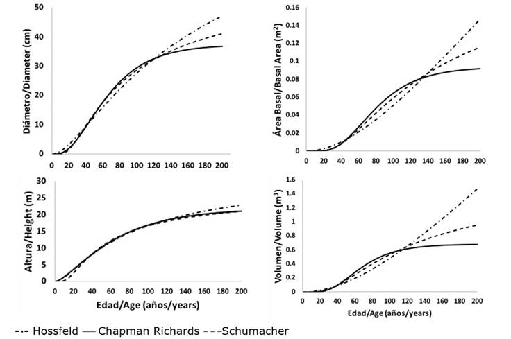
As a complement to the analysis of the results, the trends in the growth curves of the three previously selected models allowed us to determine that those of Schumacher and Chapman-Richards best represented biological growth in normal diameter, basimetric area and volume of P. leiophylla; while those of Hossfeld I and Chapman-Richards corresponded to the best trends in height growth. Schumacher’s model best characterized the growth in normal diameter, basimetric area, height and volume of both P. lumholtzii and P. strobiformis. In the latter species, the Chapman-Richards model also exhibited a good trend in height growth (Figures 2, 3 and 4).
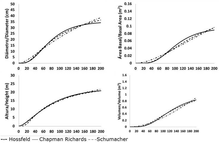
Figure 2 Trends in the average growth of normal diameter, basimetric area, height and volume of the Chapman-Richards, Hossfeld I and Schumacher models of Pinus leiophylla Schiede ex Schltdl. & Cham.
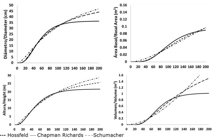
Figure 3 Trends in the average growth of normal diameter, basimetric area, height and volume of the Chapman-Richards, Hossfeld I and Schumacher models of Pinus lumholtzii B.L.Rob. & Fernand.
Current and average annual increment
Pinus lumholtzii was the species that exhibited the highest CAI max in each one of the studied variables, followed by P. strobiformis and P. leiophylla. In P. lumholtzii, the CAI max in diameter was presented at the age (t) of 30 years, much earlier than in P. leiophylla (t=55) and P. strobiformis (t=35). The age at which the CAI max was recorded in the basimetric area of P. leiophylla was higher (t=85 years) than that calculated for P. lumholtzii (E=25 years) and P. strobiformis (t=25 years) (Table 4).
Table 4 Maximum annual incremental current (CAI max ) and annual mean increment (MAI max ) estimated for each of the variables by species.
| Variable | Species | Model | CAImax | Age of
the CAImax (years) |
MAImax |
CAI-MAI Intersection (years) |
|---|---|---|---|---|---|---|
| Diameter (cm) | P. le | M1 | 0.369 | 55 | 0.249 | 95 |
| M3 | 0.349 | 45 | 0.238 | 90 | ||
| P. lu | M3 | 0.514 | 30 | 0.351 | 65 | |
| P. st | M3 | 0.444 | 35 | 0.302 | 75 | |
| Basimetric area (m2) | P. le | M1 | 0.00089 | 85 | 0.00049 | 170 |
| M3 | 0.00072 | 85 | 0.00049 | 135 | ||
| P. lu | M3 | 0.00116 | 65 | 0.00078 | 125 | |
| P. st | M3 | 0.00091 | 65 | 0.00062 | 135 | |
| Height (m) | P. le | M1 | 0.1978 | 35 | 0.16841 | 60 |
| M2 | 0.1985 | 25 | 0.16751 | 50 | ||
| P. lu | M3 | 0.3352 | 25 | 0.22932 | 55 | |
| P. st | M1 | 0.2327 | 25 | 0.20636 | 40 | |
| M3 | 0.3063 | 25 | 0.20905 | 45 | ||
| Volume (m3) | P. le | M1 | 0.00705 | 100 | 0.00438 | 160 |
| M3 | 0.00616 | 85 | 0.00418 | 170 | ||
| P. lu | M3 | 0.01156 | 75 | 0.00786 | 145 | |
| P. st | M3 | 0.00796 | 60 | 0.00541 | 115 |
P. le = Pinus leiophylla; P. lu = Pinus lumholtzii; P. st = Pinus strobiformis; M1 = Chapman-Richards model; M2 = Hossfeld I model; M3 = Schumacher model; CAI max = Maximum current annual increase; MAI max = Maximum mean annual increase.
The age at which the CAI max in height was estimated with the Hossfeld, Schumacher and Chapman-Richards models in the three species was 25 years, while the estimated age for the CAI max in volume was highest in P. leiophylla, followed by P. lumholtzii and P. strobiformis. Considering that the optimal age for defining the physical rotation of forest species happens when the CAI and the MAI in volume are equal (Mendoza, 1983), the rotation age for P. leiophylla estimated with Schumacher’s equation was 170 years, in P. lumholtzii 145 years and in P. strobiformis 115 years.
Discussion
Growth models
Similar studies have documented that the Chapman-Richards and Schumacher models are well suited for estimating the growth of individual trees. For example, Arteaga (2000) evaluated several height growth models for estimating the site index for P. radiata D. Don, P. oaxacana Mirov and P. pseudostrobus Lindl., and Monárrez and Ramírez (2003) for P. durangensis Martínez reported that Chapman-Richards’ model had the best fit.
Likewise, Corral and Návar (2005) indicated that this model is the best for estimating growth and increase in diameter, basimetric area, height and volume in five pine species in the state of Durango; while Quiñonez et al. (2015) record that this same model, in the form of algebraic differential equations, is the best for estimating growth in normal diameter of P. lumholtzii. Hernández et al. (2014), when adjusting various regression models to estimate growth in height and determine the site index for P. gregii Engelm. ex Parl., point to Schumacher’s model as the one that presented the best fit; this model also exhibited a good fit for estimating the growth in normal diameter in P. durangensis (Monárrez and Ramírez, 2003).
Current and mean annual increase
Based on the estimations of the CAI max , MAI max , the age at which the maximum annual current increase and the physical shift of each variable are attained, we infer that the species analyzed herein achieve lower CAI max or require more time than other species of the same genus to reach the maximum increases and rotation age. As evidence of the above, we cite the CAI max for normal diameter (0.75 cm), basimetric area (0.009 m2), height (0.74 m) and volume (0.048 m3) in P. herrerae Martínez (Calvillo et al., 2005); and for height in P. cooperi C.E.Blanco (0.39 m), P. durangensis (0.35 m), P. engelmanii Carr. (0.40 m, P. herrerae (0.43 m) (Corral and Návar, 2005) were superior to P. leiophylla, P. lumholtzii and P. strobiformis, species evaluated in this study.
When comparing the CAI max registered by Corral and Návar (2005) for P. leiophylla with those observed in the present research, we conclude that the CAI max in height (0.32 m vs 0.197 m) and volume were higher (0.008 m3 vs 0.007 m3), while that of the diameter (0.32 m) was lower (0.32 cm vs 0.35 cm).
When considering the age at which CAI max occurs in order to evaluate the growth of P. cooperi, P. durangensis, P. engelmanii, P. herrerae and P. leiophylla in the state of Durango, Corral and Návar (2005) determined that CAI max in diameter occurred between one and 16 years, and in height, between 19 and 24 years ―ages lower than those estimated for those variables in the three species evaluated in this study. However, the age at which the CAI max occurred in volume (70 to 105 years) was similar to that estimated by Corral and Návar (2005) for P. leiophylla, P. lumholtzii and P. strobiformis (100, 75 and 60 years, respectively).
The CAI-MAI intersection of the volume estimated by Corral and Návar (2005) for P. leiophylla is lower than that documented herein for the same species (155 years vs 160-170 years). Monárrez and Ramírez (2003) indicate that the ages at which CAI max and the physical rotation age in the diameter (t=17 years and t=35 years) and height (t=15 years and t=28 years) of P. durangensis occur were also lower than those determined for the species assessed in this study. Quiñonez et al. (2015) report that among six Pinus species, P. lumholtzii and P. leiophylla show the slowest growth in normal diameter and basimetric area; the authors argue that the slow growth that characterizes these two taxa explains the lack of interest in exploiting them economically.
Conclusions
Chapman-Richards’ and Schumacher’s models have the best fit for predicting growth in normal diameter, basimetric area and volume in P. leiophylla, while the Hossfeld I and Chapman-Richards models are the best fit to predict the growth in height. On the other hand, Schumacher’s model is best suited to predict growth in normal diameter, basimetric area, total height and volume in P. lumholtzii and P. strobiformis. The ages of the physical volume rotation age for P. leiophylla, P. lumholtzii and P. strobiformis correspond to 170, 145 and 115 years, respectively. Within the study area, these species exhibit a slow growth. The growth equations currently applied in the region of Forest Management Unit 0808 Guadalupe y Calvo, Chihuahua, should be compared with those proposed in this study in order to validate and assess their practical application.
Referencias
Arteaga M., B. 2000. Evaluación dasométrica de plantaciones de cuatro especies de pinos en Ayotoxtla, Guerrero. Revista Chapingo Serie Ciencias Forestales y del Ambiente 6(2): 151-157. https://chapingo.mx/revistas/revistas/articulos/doc/rchscfaVI335.pdf (14 de diciembre de 2019). [ Links ]
Calvillo G., J. C., E. H. Cornejo O., S Valencia M. y C. Flores L. 2005. Estudio epidométrico para Pinus herrerae Martínez en la región de Cd. Hidalgo, Michoacán México. Foresta Veracruzana 7(1): 5-10. http://www.redalyc.org/articulo.oa?id=49770102 (14 de diciembre de 2019). [ Links ]
Carmean, W. H. 1972. Site index curves for upland oaks in the Central States. Forest Science 18(2): 109-120. Doi:10.1093/forestscience/18.2.109. [ Links ]
Chávez R., N. 2009. Estudio regional forestal de la Unidad de Manejo Forestal No. 0808 “Guadalupe y Calvo, Chihuahua”. Asociación Regional de Silvicultores de Guadalupe y Calvo A. C. De De http://www.conafor.gob.mx:8080/documentos/docs/9/1147ERF_UMAFOR0808.pdf (14 de diciembre de 2009) [ Links ]
Corral R., S. y J. de J. Návar C. 2005. Análisis de crecimiento e incremento de cinco pináceas de los bosques de Durango, México. Madera y Bosques 11(1): 29-47. Doi:10.21829/myb.2005.1111260. [ Links ]
García, E. 2004. Modificación al sistema de clasificación climática de Köppen. Serie Libros 6. 5a edición. Instituto de Geografía, Universidad Autónoma de México. http://www.publicaciones.igg.unam.mx/index.php/ig/catalog/view/83/82/251-1 (14 de diciembre de 2019). [ Links ]
González M., M., F. Cruz C., G. Quiñonez B., B. Vargas L. y J. A. Nájera L. 2016. Modelos de crecimiento en altura dominante para Pinus pseudostrobus Lindl. en el estado de Guerrero. Revista Mexicana de Ciencias Forestales 7(37): 7-20. Doi:10.29298/rmcf.v7i37.48. [ Links ]
Diéguez A., U. A., A. F. Rojo, J. G. Castedo D., G. M. Álvarez, F. Barrio A., J. M. Crecente C., G. C. González, R. Pérez C., C. A. Rodríguez, M. A. López S., J. J. Balboa M., V. F. Gorgoso y R. Sánchez. 2009. Herramientas selvícolas para la gestión forestal sostenible en Galicia. Dirección Xeral de Montes, Consellería do Medio Rural, Xunta de Galicia. Galicia, España. 259 p 259 p http://mediorural.xunta.gal/fileadmin/arquivos/publicacions/herramientas_selvicolas.pdf (14 de diciembre de 2019). [ Links ]
Gizachew, B. and A. Brunner A. 2011. Density-growth relationship in thinned and unthinned Norway spruce and Scots pine stands in Norway. Scandinavian Journal of Forest Research 26(6): 543-554. Doi:10.1080/02827581.2011.611477. [ Links ]
Gyawali, A., R. P. Sharma and S. K. Bhandari. 2015. Individual tree basal area growth models pot chip pine (Pinus roxbergii Sarg) in western Nepal. Journal of Forest Science 61(12): 535-543. Doi:10.17221/51/2015-JFS. [ Links ]
Hernández R., J., J. J. García M., E. H. Olvera D., J. C. Velarde R., X. García C. y H. J. Muñoz F. 2014. Índice de sitio para plantaciones de Pinus Greggii Engelm. en Metztitlán, Hidalgo, México. Revista Chapingo Serie de Ciencias Forestales y del Ambiente 20(2): 167-176. Doi:10.5154/r.rchscfa.2013.04.016. [ Links ]
Imaña E., J. y O. Encinas B. 2008. Epidometría Forestal. Facultad de Ciencias Forestales y Ambientales de la Universidad de Brasilia, Brasil. https://repositorio.unb.br/bitstream/10482/9740/1/LIVRO_EpidometriaForestal.pdf (14 de diciembre de 2019). [ Links ]
Kiviste, A., J. G. Álvarez, G., A. Rojo A., A. D. Ruíz G. 2002. Funciones de crecimiento de aplicación en el ámbito forestal. Monografía INIA Forestal Núm. 4. Ministerio de Ciencia y Tecnología. Instituto Nacional de Investigación y Tecnología Agraria y Alimentaria (INIA). Madrid, España. 190 p. http://www.scielo.org.mx/scielo.php?script=sci_nlinks&ref=453319&pid=S1405-3195201500040000700019&lng=es (14 de diciembre de 2019). [ Links ]
Klepac, D. 1983. Crecimiento e incremento de árboles y masas forestales. Universidad Autónoma de Chapingo. Chapingo, Edo de Méx., México. 365p. http://dicifo.chapingo.mx/pdf/publicaciones/crecimiento_e_incremento_klepac_dusan.pdf (14 de diciembre de 2019). [ Links ]
López T., J. L. y J. C. Tamarit U. 2005. Crecimiento e incremento en diámetro del Lysiloma latisiliquum (L.) Benth en bosques secundarios en Escárcega, Campeche, México. Revista Chapingo Serie de Ciencias Forestales y del Ambiente 11(2): 117-123. https://chapingo.mx/revistas/forestales/contenido.php?section=article&id_articulo=438&doi (14 de diciembre de 2019). [ Links ]
Mendoza B., M. A. 1983. Conceptos básicos de manejo forestal. Ed. Limusa. México, D.F., México. 164p [ Links ]
Monárrez G., J. C. y H. Ramírez M. 2003. Predicción del rendimiento en masas de densidad excesiva de Pinus durangensis Mtz. Revista Chapingo Serie de Ciencias Forestales y del Ambiente 9(1): 45-56. https://chapingo.mx/revistas/forestales/contenido.php?section=article&id_articulo=387&doi=1111 (14 de diciembre de 2019). [ Links ]
Newberry, J. D. 1991. A note on Carmean’s estimate of height from stem analysis data. Forest Science 37(1): 368-369. Doi:10.1093/forestscience/37.1.368. [ Links ]
Piennar, L. V. and J. W. Rheney. 1995. Modeling stand level growth and yield response to silvicultural treatments. Forest Science 41(3): 629-638. Doi:10.1093/forestscience/41.3.629. [ Links ]
Quiñonez B., G., H. M. De los Santos P. y J. G. Álvarez G. 2015. Crecimiento en diámetro para Pinus en Durango. Revista Mexicana de Ciencias Forestales 6(29): 108-125. Doi:10.29298/rmcf.v6i29.220. [ Links ]
Quiñonez B., G., G. G. García E. y O. A. Aguirre C. 2018. ¿Cómo corregir heterocedasticidad y autocorrelación de residuales en modelos de ahusamiento y crecimiento en altura? Revista Mexicana de Ciencias Forestales 9(49): 28-59. Doi:10.29298/rmcf.v9i49.151. [ Links ]
Torres R., J. M. y O. S. Magaña T. 2001. Evaluación de plantaciones forestales. CIDE, Limusa, Noriega Editores. México, D.F., México. 472p. [ Links ]
Salazar G., J. G., J. J. Vargas H., J. Jasso M., J. D. Molina G., C. Ramírez H. y J. López U. 1999. Variación en el patrón de crecimiento en altura de cuatro especies de Pinus en edades tempranas. Madera y Bosques 5(2): 19-34. Doi:10.21829/myb.1999.521345. [ Links ]
Sharma, R. P., A. Brunner, T. Eid and B. H. Øyen. 2011. Modelling dominant height growth from national forest inventory individual tree data with short time series and large age errors. Forest Ecology and Management 262(12): 2162-2175. Doi:10.1016/j.foreco.2011.07.037. [ Links ]
Statistical Analysis System (SAS). 2002. SAS Version 8. SAS Institute Inc. Cary, NC. USA. n/p. [ Links ]
Valdéz L., R. J. y T. B. Lynch. 2000. Ecuaciones para estimar volumen comercial y total en rodales aclareados de Pinus patula en Puebla, México. Agrociencia 34(6): 747-758. https://www.colpos.mx/agrocien/Bimestral/2000/nov-dic/art10.pdf (14 de diciembre de 2019). [ Links ]
Zimmerman, D. L., V. Nuñez A., T. G. Gregoire, O. Schabenberger, J. D. Hart, M. G. Kenward, G. Molenberghs, G. Verbeke, M. Pourahmadi and P. Vieu. 2001. Parametric modelling of growth curve data: An overview. Sociedad de Estadística e Investigación Operativa Test 10(1): 1-73. Doi:10.1007/BF02595823. [ Links ]
Received: December 09, 2019; Accepted: April 30, 2020
 Este es un artículo publicado en acceso abierto bajo una licencia
Creative Commons
Este es un artículo publicado en acceso abierto bajo una licencia
Creative Commons
