


Serviços Personalizados
Journal
Artigo
 texto em
  Inglês (pdf)
 Artigo em XML
 Referências do artigo
 Enviar este artigo por email
Indicadores
-
 Citado por SciELO
 -
 Acessos
Links relacionados
-
 Similares em
SciELO
Similares em
SciELO
Compartilhar

 Permalink
Revista mexicana de ciencias forestales
versão impressa ISSN 2007-1132
Rev. mex. de cienc. forestales vol.9 no.50 México Nov./Dez. 2018
https://doi.org/10.29298/rmcf.v9i50.261
Articles
Volume equations for Prosopis articulata S. Watson and Lysiloma divaricata (Jacq.) J. F. Macbr. in northwestern Mexico
1Facultad de Ciencias Forestales, Universidad Autónoma de Nuevo León. México.
Allometric models are a tool of great importance for forest management, as they allow reliable estimations of the volume of both individual trees and forest stands, as well as the construction of volume tables in order to facilitate the quantification of timber stocks. In the present work, data of 160 trees were adjusted; 80 trees of each species were cut, covering all the diameter categories; the variables measured were: normal diameter (D), base diameter (DB) total height (H), and crown diameter (DC), as well as the diameters and lengths of each of the branches with a diameter above 6 cm at its base. Linear, multiple and nonlinear regression models with one and two independent variables were tested to estimate the total stem volume with bark. For the selection of the best model, the RMSE, adjusted R2 and the level of significance of the parameters were taken into account. For the prediction of the total volume according to the normal diameter, the allometric model of Berkhout presented better adjustments, with R2 of 0.9053 and RMSE of 0.0432 for Prosopis articulata and R2 of 0.8178, as well as RMSE of 0.1048 for Lysiloma divaricata. Using the variables normal diameter and total height, the best adjustments were obtained with the Schumacher-Hall model, with values of 0.9139 in R2 and RMSE of 0.0411 for Prosopis articulata. For Lysiloma divaricata the best fit model was the Spurr potential with R2 of 0.7936 and a value of RMSE of 0.1118.
Key words: Diametric categories; forest management; model; prediction; volume tables; volume
Una herramienta de gran importancia en el manejo forestal son los modelos alométricos, con los cuales se puede estimar de forma confiable el volumen en árboles individuales y masas forestales, además de construirse tablas de volumen que faciliten la cuantificación de existencias maderables. En el presente trabajo se ajustaron datos de 160 árboles; para ello, se derribaron 80 individuos de cada especie que incluyeron todas las categorías diamétricas. Se midieron las variables: diámetro normal (D), diámetro de la base (DB) altura total (H) y diámetro de copa (DC), así como los diámetros y longitudes de cada una de las ramas mayores a 6 cm de diámetro en su base. Se probaron modelos de regresión lineal simple, múltiple y no-lineal con una y dos variables independientes, para estimar el volumen fustal total con corteza. La selección del mejor modelo se hizo con base en la RCME, R2 ajustado y el nivel de significancia de los parámetros. Para la predicción del volumen total en función del diámetro normal, el modelo alométrico de Berkhout presentó mejores ajustes, con R2 de 0.9053 y RCME de 0.0432 para Prosopis articulata; y R2 de 0.8178, RCME de 0.1048 para Lysiloma divaricata. A partir del diámetro normal y altura total, los mejores ajustes se obtuvieron con el modelo de Schumacher-Hall, con valores de 0.9139 en R2 y RCME de 0.0411 para Prosopis articulata; para Lysiloma divaricata el modelo de mejor ajuste fue el Spurr Potencial con R2 de 0.7936 y un valor de RCME de 0.1118.
Palabras clave: Categorías diamétricas; manejo forestal; modelo; predicción; tablas de volumen; volumen
Introduction
The importance of generating biometric systems lies in the integration of static or dynamic statistical mathematical models for a rational, sustainable management of forests. Today these models are the most widely used analytical tools for generating knowledge about the production and growth of forest masses (Weiskittel et al., 2011; Vargas-Larreta et al., 2017). This is achieved by measuring certain variables, such as the normal diameter and the total height; subsequently estimating the volume of each tree, and, finally, extrapolating the information to a whole stand (Acosta-Mireles and Carrillo-Anzures, 2008; Cruz-Cobos et al., 2016).
Simulation with mathematical models is helpful for making decisions in sustainable forest management. Volume models predict the total volume of trees with and without bark, as well as of the clean trunk, total stem and commercial stem; furthermore, it is the main method for the construction of prices or volume tables (Schumacher and Hall, 1933; Tapia and Návar, 2011).
Volume equations and their tabulated expressions are one of the main tools for gaining reliable knowledge of the actual stocks and carrying out sustainable management. They are also helpful for forest management, the commercialization of timber products, and research, particularly in the form or seasonal quality studies (Muñoz-Flores et al., 2003; Velasco et al., 2010).
The timber exploitation of Prosopis articulata S. Watson (mesquite) and Lysiloma divaricate (Jacq.) J. F. Macbr. (mauto) is a forest activity in the arid and semiarid areas of northern Mexico (León-De la Luz et al., 2008; Rodríguez-Sauceda et al., 2014). Despite the importance of the forest resources of these regions, very little detailed research has been carried out so far to accurately assess the estimates of volume production at species level.
The objective of the present research is to develop a volume system for the two species with the highest forest importance -Prosopis articulata and Lysiloma divaricata- in Southern Baja California, Mexico. The information to be thus obtained will serve as a basis for the silvicultural management of arid forest masses in the study region.
Materials and Methods
Study area
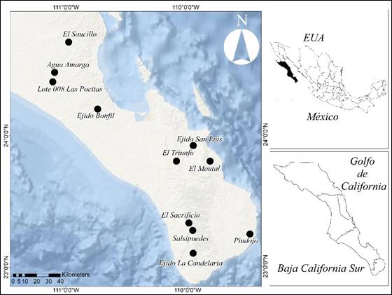
The study was carried out in plots that belong to a Forest Management Unit (Umafor) 303, located in the south of Southern Baja California, includes two municipalities: La Paz and Los Cabos (Figure 1) and is managed by the Sierra La Laguna Association of Forest Producers, A.C.
According to Köppen’s classification modified by García (1988); the dominant climate is very dry, semiarid (BWh), followed by very dry, warm (BW(h'), dry semiarid (BSh), and only the area of Sierra La Laguna has temperate climates, such as temperate subhumid with summer rains with less humidity C(w0), and temperate subhumid with summer rains and medium humidity C(w1).
The physical factors of the environment favor the development of different vegetation types along an altitude gradient (Arriaga and Ortega, 1988), characterized by xerophilous shrubs, represented by sarcocaule shrubs, sarcocrassicaule shrubs, low deciduous forest, low subdeciduous forest, and gallery vegetation.
The topography corresponds to mountain chains, plains, hills, beaches, plateaus and ravines.
In-field assessment
Privately owned plots and communal lands (ejidos) with timber potential were selected as sources of the dasometric data required for the study, using a destructive sampling, which consisted in felling, sectioning and measuring the trees chosen through directed sampling -of 80 individuals per species-, and in which the qualities of the season and the categories of diameter and height were represented.
The following variables were measured: normal diameter with bark (D), total height (H) and diameters at different heights with bark (d). The height from the ground level (h) was recorded for each of the sections. Diameters were measured at the base of branches with a diameter above 6 cm, with and without bark; smaller diameters were not included because they lack commercial interest. The total height was measured with a Suunto Pm5/360pc clinometer; and to obtain the different diameters a 122450 Ben Meadows diameter tape was used.
The felled trees were cut to a maximum stump height of 0.30 m above the ground level; next, two sections -each with a length of 0.30 cm- were cut above the stump. The next corresponded to the normal diameter (1.30 m); 0.50 m long sections were subsequently obtained, up to the tip of the tree (Figure 2). Two perpendicular diameters were considered in each, with and without bark, and the mean diameter was estimated.
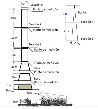
Sección = Section; Punto de medición = Measuring point; Base = Base.
Figure 2 Graphic representation of the measuring points at the various sections of the tree.
Based on the characteristics described above, each of the sections of the trunk was cubed, from the stem to the branches, using Smalian’s formula:
Where:
𝑉 = Volume of the section (m³)
d1 = Larger diameter (m)
d2 = Smaller diameter (m)
𝐿 = Length (m)
The total volume of the tree was calculated based on the sum of all the volumes estimated for each section of the tree.
Analysis of the information
25 simple, multiple allometric, linear and non-linear regression models were adjusted with one (Table 1), two or three predictive variables, respectively (Table 2), by applying the minimum ordinary squares method (MOS) and weighted least squares (WLS) with the SAS statistical software package (SAS, 1990).
Table 1 One-variable models evaluated in order to estimate the volume of mesquite and mauto.
| Model | Name | Expression |
|---|---|---|
| M1 | Dissescu-Stanescu (second degree incomplete polynomial) |
|
| M2 | Berkhout (allometric) |
|
| M3 | Dissescu-Meyer |
|
| M4 | Hohenadl-Krenn (second degree complete polynomial) |
|
| M5 | Dissescu-Stanescu (second degree incomplete polynomial) (Mod. Var. DB) |
|
| M6 | Berkhout (allometric ) (Mod. Var. DB) |
|
| M7 | Dissescu-Meyer (Mod. Var. DB) |
|
| M8 | Hohenadl-Krenn (second degree complete polynomial) (Mod. Var. DB) |
|
| M9 | Dissescu-Stanescu (second degree incomplete polynomial) (Mod. Var. H) |
|
| M10 | Berkhout (allometric) (Mod. Var. H) |
|
| M11 | Dissescu-Meyer (Mod. Var. H) |
|
| M12 | Hohenadl-Krenn (second degree complete polynomial) (Mod. Var. H) |
|
| M13 | Dissescu-Stanescu (second degree incomplete polynomial) (Mod. Var. DC) |
|
| M14 | Berkhout (allometric) (Mod. Var. DC) |
|
| M15 | Dissescu-Meyer (Mod. Var. DC) |
|
Table 2 Models with two or more independent variables evaluated for estimating the volume of mesquite and mauto.
| Model | Name | Expression |
|---|---|---|
| M16 | Schumacher-Hall |
|
| M17 | Spurr |
|
| M18 | Spurr potential |
|
| M19 | Spurr with independent term |
|
| M20 | Generalized incomplete combined variable |
|
| M21 | Undefined |
|
| M22 | Spurr with independent term (Mod.) |
|
| M23 | Undefined |
|
| M24 | Undefined |
|
| M25 | Undefined |
|
Source: Cruz-Cobos et al., 2016; Vargas-Larreta et al., 2017.
V = Volume (m3); D = Normal diameter (cm); H = Total height (m); DB = Diameter at base (cm); CD = Crown diameter (m); NB = Number of branches; VC = Squared base diameter ratio (cm) multiplied by the height (m); 𝛽0, 𝛽1, 𝛽2, 𝛽3 = Parameters to be estimated.
The quality of the adjustment of the models was assessed using graphic and numeric analysis, based on the highest value for the adjusted coefficient of determination (adjusted R2), the lowest value for the root mean square error (RMSE), the graphic representations, and the level of significance of the parameters according to Vargas-Larreta et al. (2017).
Where:
n = Number of observations
p = Number of parameters
Torres-Rojo and Magaña-Torres (2001), as well as Cruz-Cobos et al. (2016), point out that most volume models exhibit heteroscedasticity issues because the variation in the volume of the trees increases in direct proportion to the values of diameter and height, and corrections with weighted least squares are therefore required.
The graphical analysis of the studentized residuals versus the estimated values using the selected models evidenced heteroscedasticity issues; for this reason, they had to be corrected through weighted regression, with the weighted least squares method. The ordinary least squares method is employed to estimate the regression line, which seeks to minimize the sum of squared errors; i.e. each error receives an equal weighting, whether or not it stems from an observation with a higher or a lower variance. Conversely, the weighted least squares method adds more weight to those observations that exhibit a lower standard deviation than to those with a higher one, allowing a more accurate estimation of the regression line.
Results and Discussion
Table 3 shows the basic descriptive statistics of the variables considered in the models for Prosopis articulata and Lysiloma divaricata; the adjustment of the models was observed to cover a broad interval of the independent variables utilized.
Table 3 Descriptive statistics for the database for Prosopis articulata S.Watson and Lysiloma divaricata (Jacq.) J.F.Macbr.
| Variable | P. articulata statistics | L. divaricata statistics | ||||||
|---|---|---|---|---|---|---|---|---|
| Maximum | Minimum | Mean | SD | Maximum | Minimum | Mean | SD | |
| D | 42.5 | 7.6 | 23.96 | 9.55 | 41 | 8.9 | 24.18 | 9.43 |
| H | 10.58 | 3.53 | 6.50 | 1.57 | 12.2 | 3.5 | 9.46 | 2.31 |
| DB | 52 | 11.5 | 29.24 | 10.63 | 53.5 | 10 | 28.91 | 11.27 |
| CD | 8.5 | 1 | 3.65 | 1.86 | 13 | 1.5 | 5.08 | 2.93 |
| NB | 7 | 0 | 1.17 | 1.11 | 1.10 | 0.02 | 0.29 | 0.24 |
| VT | 0.60 | 0.013 | 0.18 | 0.13 | 3 | 0 | 1.77 | 1.02 |
VT = Volume (m3); D = Normal diameter (cm); H = Total height (m); DB = Diameter at base (cm); CD = Crown diameter (m); NB = Number of branches.
Figure 3 shows the tendency of the volume-normal diameter and volume-total height pairs of data for Prosopis articulata. The sample size for each diameter category varied due to the abundance of trees of certain dimensions in the study area; diameters of 7.6 to 42.5 cm were included, the most frequent being those between 10 and 30 cm. Likewise, the most frequent heights ranged between 5 and 10 m.
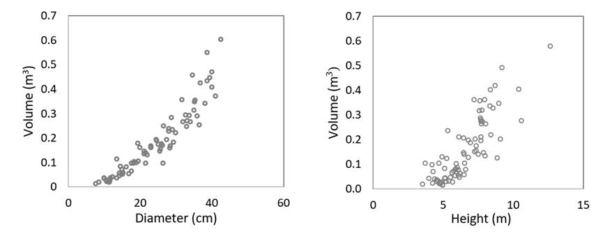
Figure 3 Dispersion graphs of the volume-diameter (left) and volume-height (right) data pairs for Prosopis articulata S.Watson.
Figure 4 shows the tendency of the volume-normal diameter and volume-total height data pairs for Lysiloma divaricata. Diameters of 8.9 to 41 cm were considered, of which the most frequent ranged between 10 and 30 cm; the heights were of 5 to 12 m.
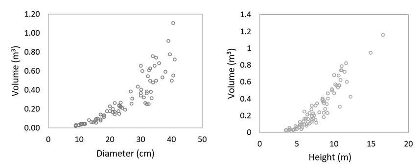
Figure 4 Dispersion graphs of the volume-diameter and volume-height for Lysiloma divaricata (Jacq.) J.F.Macbr.
Table 4 summarizes the goodness-of-fit statistics of the volume model of a variable for Prosopis articulata. The highest values for R2 and the lowest for RMSE were obtained using those models whose independent variable is the normal diameter (M1-M4).
Table 4 Goodness-of-fit statistics of the one-variable model Prosopis articulata S. Watson.
| Equation | R2 | RMSE | Bias |
|---|---|---|---|
| M1 | 0.90527794 | 0.0428437 | -0.0064217 |
| M2 | 0.90545388 | 0.04280389 | -0.0049428 |
| M3 | 0.90531866 | 0.04283449 | -0.0057673 |
| M4 | 0.90558798 | 0.04305038 | -0.0064217 |
| M5 | 0.67344067 | 0.07955041 | -0.0064217 |
| M6 | 0.67382001 | 0.0795042 | -0.0066161 |
| M7 | 0.67386939 | 0.07949818 | -0.0067407 |
| M8 | 0.67431109 | 0.07995853 | -0.0064217 |
| M9 | 0.47238585 | 0.10111594 | -0.0012141 |
| M10 | 0.46996466 | 0.10134768 | -0.0032696 |
| M11 | 0.47050001 | 0.10129648 | -0.0021356 |
| M12 | 0.50162254 | 0.09891053 | -0.0019025 |
| M13 | 0.52686768 | 0.09575307 | -0.0064217 |
| M14 | 0.53692929 | 0.09472946 | -0.0054247 |
| M15 | 0.53827914 | 0.09459129 | -0.0036454 |
The analysis of the residuals of model M2, selected as the best for estimating the volume of Prosopis articulata trees, exhibited a tendency to increase in direct proportion to the predicted volume. The correction was made using weighted regression.
Table 5 shows the goodness-of-fit statistics and estimators of the parameters of Berkout’s Allometric Model (M2) for Prosopis articulata.
Table 5 Goodness-of-fit statistics for Prosopis articulata S. Watson corrected with weighted least squares using Model 2.
| Equation | R2 | RMSE | Bias | Parameters | |
|
|
|
||||
| M2 | 0.9054 | 0.04280 | -0.0049428 | 0.000239 | 2.04015 |
The two-variable volume models for Prosopis articulata exhibited greater adjustments than those that consider a single independent variable; those involving the diameter and height as independent variables resulted in slight improvements; only a few failed to attain the selected level of significance (5 %). Table 6 shows the statistics of Model 16, which had the highest R2, the lowest RMSE, almost zero bias, and significant parameters; for these reasons it was selected for the estimation of the volume of P. articulata.
Table 6 Goodness-of-fit statistics and parameters of the models with two and three independent variables for Prosopis articulata S. Watson.
| Equation | R2 | RMSE | Bias |
|---|---|---|---|
| M16 | 0.9186 | 0.0400 | 0.00022 |
| M17 | 0.8838 | 0.0471 | 0.01417 |
| M18 | 0.8574 | 0.0525 | -0.00043 |
| M19 | 0.9024 | 0.0435 | -0.00032 |
| M20 | 0.9075 | 0.0425 | -0.00022 |
| M21 | 0.8057 | 0.0617 | 0.00132 |
| M22 | 0.7974 | 0.0627 | -0.00003 |
| M23 | 0.9050 | 0.0431 | -0.05745 |
| M24 | 0.9024 | 0.0435 | -0.06197 |
| M25 | 0.9176 | 0.0405 | -0.00005 |
The graphic analysis of the residuals of Model 16 for Prosopis articulata evidenced the presence of heteroscedasticity. Furthermore, the residuals were corrected using the weighted least squares method.
Arter the correction of the heteroscedasticity, Table 7 shows the statistics and adjusted parameters of Shumacher-Hall’s model for the estimation of the volume of Prosopis articulata.
Table 7 Adjustment statistics of Model 16, corrected using weighted least squares, for Prosopis articulata S. Watson.
| Model | R2 | RMSE | Bias | Parameters | ||
|
|
|
|
||||
| M16 | 0.9139 | 0.0411 | 0.00022 | 0.0002 | 1.8881 | 0.4061 |
Table 8 shows the goodness-of-fit statistics of the one entry volume models for Lysiloma divaricata. The highest R2 values and the lowest RMSE values were obtained using those models that include the normal diameter (M1-M4), followed by those that considered the diameter at base (M5-M8). Conversely, the adjustments of those models that include the total height of the trees and the crown diameter were less efficient.
Table 8 Goodness-of-fit statistics and parameters of the one entry model for Lysiloma divaricata (Jacq.) J. F. Macbr.
| Model | R2 | RMSE | Bias |
|---|---|---|---|
| M1 | 0.8287 | 0.1019 | 2.0052E-10 |
| M2 | 0.8294 | 0.1016 | -0.000427 |
| M3 | 0.8293 | 0.1017 | 0.00035825 |
| M4 | 0.8294 | 0.1023 | 3.9996E-11 |
| M5 | 0.6795 | 0.1393 | -5.649E-10 |
| M6 | 0.6918 | 0.1366 | 0.28615368 |
| M7 | 0.6853 | 0.1381 | -0.0062446 |
| M8 | 0.7150 | 0.1322 | 1.7601E-10 |
| M9 | 0.5821 | 0.1591 | -4.627E-11 |
| M10 | 0.5780 | 0.1599 | -0.005714 |
| M11 | 0.5799 | 0.1595 | -0.0023334 |
| M12 | 0.5919 | 0.0985 | 8.7213E-11 |
| M13 | 0.4518 | 0.1822 | -8.223E-17 |
| M14 | 0.4191 | 0.1876 | 0.0069449 |
| M15 | 0.4208 | 0.1873 | 0.01102998 |
The graphic analysis of the studentized residuals versus the estimated values of Model 2 showed the absence of homogeneity in the values of the variances, corrected by means of weighted regression.
After the correction of the heteroscedasticity, the final results of the adjustment to Berkout’s Allometric Model (M2) exhibits the adjustment statistics and the parameters shown in Table 9.
Table 9 Adjustment statistics for Lysiloma divaricata (Jacq.) J. F. Macbr. for Model 2 (M2), corrected using the Weighted Least Squares method.
| Model | R2 | RMSE | Bias | Parameters | |
|
|
|
||||
| M2 | 0.8294 | 0.1016 | -0.000427 | 0.0002 | 2.2339 |
Those models that consider two predictive variables -e.g. diameter and height (M16-M25)- evidenced adjustments above those of the models that consider a single independent variable (diameter), with R2 values ranging between 0.75 and 0.86,and RMSE values of 0.09 to 0.1. However, some models fail to attain the necessary level of significance (5 %) (Table 10), and therefore Model 18 was selected, due to its good fit and to the significance level of the parameter estimators.
Table 10 Goodness-of-fit statistics of the model with two and three entries for Lysiloma divaricata (Jacq.) J. F. Macbr.
| Equation | R2 | RMSE | Bias |
|---|---|---|---|
| M16 | 0.8336 | 0.1010 | -0.0010269 |
| M17 | 0.8044 | 0.1081 | 0.01737528 |
| M18 | 0.7977 | 0.1107 | -0.0026761 |
| M19 | 0.8162 | 0.1055 | 0.00106051 |
| M20 | 0.8167 | 0.1060 | -0.0005477 |
| M21 | 0.8625 | 0.0919 | -0.0035862 |
| M22 | 0.6786 | 0.1395 | -0.0031733 |
| M23 | 0.8625 | 0.0919 | -0.0035862 |
| M24 | 0.6786 | 0.1395 | -0.0031733 |
| M25 | 0.6786 | 0.1395 | 6.7808E-10 |
Like the previously analyzed models, M18 the Spurr potential model with one combined variable for Lysiloma divaricata exhibited heteroscedasticity, which was corrected using the WLS method. Table 11 shows the final adjustment statistics of the corrected M18.
Table 11 Adjustment statistics for mauto, corrected using weighted least squares, with Model 18 for Lysiloma divaricata (Jacq.) J. F. Macbr.
| Model | R2 | RMSE | Bias | Parameters | |
|
|
|
||||
| M18 | 0.7977 | 0.1107 | -0.0026761 | 0.0001 | 1.363298 |
The best adjustments for one entry models for Prosopis articulata and Lysiloma divaricata were obtained using M2, whose independent variable is the normal diameter. These results agree with those obtained by Rodríguez et. al. (2012), who carried out a study in a cloud forest in Tamaulipas, Mexico, in which they adjusted models for broadleaf and conifer species and concluded that Berkhout’s allometric model has a very good fit and is reliable for the estimation of total stem volumes based on the normal diameter. Furthermore, the results of the research documented herein agree with those of Cruz et al. (2016), according to whom Berkhout’s allometric model with the diameter variable and Shumacher-Hall’s model with the independent variables diameter and height had the best fit for the estimation of volumes for Arbutus spp. in the region of Pueblo Nuevo, Durango, Mexico (Figure 5).
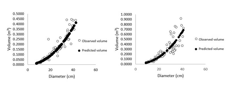
Figure 5 Graphic representation of the volume estimated using Berkhout’s one entry model for Prosopis articulata S. Watson (left) and Lysiloma divaricata (Jacq.) J. F. Macbr. (right).
Conversely, Hernández-Herrera et al. (2014) adjusted a series of regression models based on a sample of 38 trees using various predictive variables in the selection and adjustment of their best volume estimation.
Vargas-Larreta et al. (2017) compared models in order to predict the total volume of several timber species in different states of the Mexican Republic, based on the normal diameter and the total height; their results agree with those obtained in this study, in the sense that Shumacher-Hall’s model exhibited the best adjustments. This model is widely used to estimate the total volume, both in conifers and in broadleaves. Da Cunha and Guimarães-Finger (2009) adjusted a series of regression models and selected the Spurr potential model for developing a double-entry volume table for Pinus taeda L. in southern Brazil.
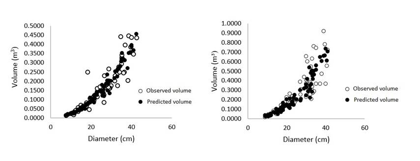
The best fits for the two-entry models for Prosopis articulata and Lysiloma divaricata were obtained using the independent variables normal diameter and total height. The models selected for the estimations were M16 -i.e. Shumacher-Hall’s, and M18, the Spurr potential model- for the simplicity of their implementation and structure (Figure 6).
Conclusions
The independent variable normal diameter produced the best adjustments using Berkhout’s Allometric Model (M2) for Prosopis articulata and Lysiloma divaricata, since this model allows a reliable estimation of the volume; however, Shumacher-Hall’s combined variable model was the one with the best fit in the estimation of the total volume of Prosopis articulata, while the Spurr potential model produced the best fit for the estimation of the total stem volume of Lysiloma divaricata. These two models yield reliable, accurate estimates, as their structure includes an additional variable.
Acknowledgments
To the Comisión Nacional Forestal Baja California Sur (South Baja California National Forest Commission) for the funding provided to accomplish this project, as well as to ASAMYFOR SC company for the technical support during field work
REFERENCES
Acosta-Mireles, M. y F. Carrillo-Anzures. 2008. Cuadro de volumen total con y sin corteza para Pinus montezumae Lamb. en el estado de Hidalgo. Folleto Técnico Núm. 7. INIFAP. Campo Experimental Pachuca. Pachuca, Hgo., México 20 p. [ Links ]
Arriaga, L. y A. Ortega. (eds.). 1988. La Sierra de La Laguna en Baja California Sur, Centro de Investigaciones Biológicas de Baja California A.C. La Paz, B.C.S., México. 237 p. [ Links ]
Cruz-Cobos, F., R. Mendía-Santana., A. Jiménez-Flores., J. Nájera-Luna y F. Cruz-García. 2016. Ecuaciones de volumen para Arbutus spp. (madroño) en la región de Pueblo Nuevo, Durango. Investigación y Ciencia 24(68): 41-47. [ Links ]
da Cunha, T. A. y C. A. Guimarães-Finger. 2012. Modelo de regresión para estimar el volumen total con corteza de árboles de Pinus taeda L. en el sur de Brasil. Revista Forestal Mesoamericana Kurú 6(16): 26-40. [ Links ]
Fuentes-Salinas, M., F. Correa-Méndez., y A. Corona-Ambriz. 2008. Características tecnológicas de 16 maderas del estado de Tamaulipas, que influyen en la fabricación de tableros de partículas y de fibras. Revista Chapingo Serie Ciencias Forestales y del Ambiente 14(1): 65-71. [ Links ]
García, E. 1988. Atlas climático de la República Mexicana. Ed. Porrúa. México, D.F., México. 250 p. [ Links ]
Hernández-Herrera, J., L. Valenzuela-Núñez., A. Flores-Hernández y J. Ríos-Saucedo. 2014. Análisis dimensional para determinar volumen y peso de madera de mezquite (Prosopis L.). Madera y Bosques 20(3):155-161. [ Links ]
León-de la Luz, J., R. Domínguez-Cadena y S. Díaz-Castro. 2005. Evaluación del peso del leño a partir de variables dimensionales en dos especies de mezquite Prosopis articulata S. Watson y P. palmeri S. Watson, en Baja California Sur, México. Acta Botánica Mexicana 72:17-32. [ Links ]
Muñoz-Flores, H., S. Madrigal H., M. Aguilar R., J. García M. y M. Lara R. 2003. Tablas de volumen para Pinus lawsonii Roezl y P. pringlei Shaw. en el Oriente de Michoacán. Ciencia Forestal en México 28(94):81-104. [ Links ]
Rodríguez-Sauceda, E., G. Rojo-Martínez., B. Ramírez-Valverde., R. Martínez-Ruiz., M. Cong-Hermida., S. Medina-Torres y H. Piña-Ruiz. 2014. Análisis técnico del árbol del mezquite (Prosopis laevigata Humb. & Bonpl. ex Willd.) en México. Ra Ximhai 10(3):173-193. [ Links ]
Rondeux, J. 2010. Medición de árboles y masas forestales. Ediciones Mundi-Prensa. Madrid, España. 521 p. [ Links ]
Statistical Analysis System (SAS). 1990. SAS/STAT user's guide: version 6 (Vol. 2). SAS Institute. Cary, NC, USA. n/p. [ Links ]
Schumacher, F. X. and F. D. S. Hall. 1933. Logarithmic expression of timber-tree volume. Journal of Agricultural Research 47:719-734. [ Links ]
Tapia, J. y J. Návar. 2011. Ajuste de modelos de volumen y funciones de ahusamiento para Pinus pseudostrobus Lindl. en bosques de pino de la Sierra Madre Oriental de Nuevo León, México. Foresta Veracruzana 13(2): 19-28 [ Links ]
Torres-Rojo, J. y O. Magaña-Torres. 2001. Evaluación de Plantaciones Forestales. Ed. Limusa. México, D.F., México. 473 p. [ Links ]
Vargas-Larreta, B., J. Corral-Rivas., O. Aguirre-Calderón., J. López-Martínez., H. De los Santos-Posadas., F. Zamudio-Sánchez., E. Treviño-Garza., M. Martínez-Salvador y C. Aguirre-Calderón. 2017. SiBiFor: Forest Biometric System for forest management in Mexico. Revista Chapingo Serie Ciencias Forestales y del Ambiente 23(3): 437-455. [ Links ]
Velasco B., E., S. Madrigal H., I. Vázquez C., A. González H. y F. Moreno S. 2006. Manual para la elaboración de tablas de volumen fustal en pino. Libro Técnico Núm. 1. INIFAP-Conacyt-Conafor. México, D.F. México. 34 p. [ Links ]
Weiskittel, A. R., Hann, D. W., Kershaw, J. A. and Vanclay J. K. 2011. Forest growth and yield modeling. Wiley-Blackwell Press. West Sussex, UK. 416 p. [ Links ]
Received: March 22, 2018; Accepted: September 24, 2018
 Este es un artículo publicado en acceso abierto bajo una licencia Creative Commons
