


Services on Demand
Journal
Article
 text in
  English (pdf)
 Article in xml format
 Article references
 Send this article by e-mail
Indicators
-
 Cited by SciELO
 -
 Access statistics
Related links
-
 Similars in
SciELO
Similars in
SciELO
Share

 Permalink
Revista mexicana de ciencias forestales
Print version ISSN 2007-1132
Rev. mex. de cienc. forestales vol.9 n.48 México Jul./Aug. 2018
https://doi.org/10.29298/rmcf.v8i48.114
Articles
The ecological niche as a tool for predicting potential areas of two pine species
1Campo Experimental Centro de Chiapas, Centro de Investigación Regional Pacífico Sur, INIFAP. México.
2División de Ciencias Forestales, Universidad Autónoma Chapingo. México.
3Campo Experimental Chetumal, Centro de Investigación Regional Sureste, INIFAP. México.
4Campo Experimental Uruapan, Centro de Investigación Regional Pacífico Centro, INIFAP. México.
5Departamento de Germoplasma Forestal, Gerencia Estatal Chiapas, Conafor. México.
Modelling the optimum ecological niche after the species potential distribution, a tool to predict potential production sites is an option for delimitation of best seed stands as Forest Germplasm Production Areas (UPGF) The aim of this study was to model the potential distribution of Pinus pseudostrobus and P. oocarpa in Chiapas, Mexico by mapping topographic, climatic, edaphic, ecological and ecological niche models (MaxEnt). Data for 220 site presence points for P. oocarpa and 52 for P. pseudostrobus were obtained from the World Information Network on Biodiversity, Global Biodiversity Information Facility, the Missouri Botanical Garden and Herbario Nacional de México [National Herbarium of Mexico (MEXU)]. The potential distribution for each species was modelled after 500 and 1 000 iterations through Logistic, Cumulative and Cloglog regressions. Statistical validation was performed with 28 % of the data for each species through the technique Crossvalidate and Bootstrap. The best fit model was the Logistic type with crossvalidate type validation. Values of area down the curve (AUC) for estimated and validated data were 0.882 (P. oocarpa) and 0.947 (P. pseudostrobus). The most influent variables for species presence or absence were altitude with 84.5 y 97.3 % for P. oocarpa and P. pseudostrobus, respectively. Results from the best model allowed the delimitation of optimum sites to establish UPGF.
Key words: AUC; Chiapas; forest germplasm; MaxEnt; predictive models; Forest Germplasm Production Areas
Modelar el nicho ecológico óptimo para determinar la distribución potencial de las especies es una opción viable en la ubicación de las mejores áreas para establecer Unidades Productoras de Germoplasma Forestal (UPGF). El objetivo del presente estudio fue modelar la distribución potencial de Pinus pseudostrobus y P. oocarpa en Chiapas, México, mediante el procesamiento cartográfico de variables topográficas, climáticas, edáficas, ecológicas y modelos de nicho ecológico (MaxEnt). Se utilizaron 220 datos de presencia de P. oocarpa y 52 para P. pseudostrobus obtenidos de la Red Mundial de Información sobre Biodiversidad, Global Biodiversity Information Facility, del Missouri Botanical Garden y del Herbario Nacional de México (MEXU). La distribución potencial de la especie fue modelada con 500 y 1 000 iteraciones a través de las regresiones de tipo Logistic, Cumulative y Cloglog. La validación estadística se realizó con 28 % de los datos para cada taxón con las técnicas Crossvalidate y Bootstrap. El modelo que mejor se ajustó fue el logístico con método de remuestreo crossvalidate. Los valores del Área Bajo la Curva (AUC) para los datos estimados y validados fueron de 0.882 para P. oocarpa y 0.947 en P. pseudostrobus. La variable que más influyó en la presencia o ausencia de las especies fue la altitud con 84.5 y 97.3 % para P. oocarpa y P. pseudostrobus, respectivamente. Los resultados del modelo permitieron ubicar áreas óptimas para el establecimiento de UPGF.
Palabras clave: AUC; Chiapas; germoplasma forestal; MaxEnt; modelos predictivos; Unidades Productoras de Germoplasma Forestal
Introduction
The forest germplasm used in Mexico in the production of seedlings to supply the national reforestation programs comes from natural populations or from unmanaged forest plantations, in which the phenotypic and genotypic quality of the individuals for their collection is not considered (Muñoz et al., 2014). In addition, part of the plant produced is used indiscriminately for the reforestation of areas in edaphoclimatic conditions different from the areas of germplasm origin (Secretaría de Economía, 2016).
The wrong selection of this material and the inadequate use of the plants produced have an impact on the survival, production and yield of reforestation or commercial forest plantations (PFC) (Alba et al., 2005). On the other hand, by introducing forest plants in areas under environmental conditions completely different from those required by each species, they can become vectors of pests and diseases (Vanegas, 2016), alter trophic relationships and cause loss of biodiversity (Fernández-Pérez et al., 2013).
Since 2001, the Comisión Nacional Forestal (National Forestry Commission) (Conafor) has promoted reforestation for the ecological restoration of degraded areas (Vanegas, 2016). A key factor for the success of reforestations is the management and production of forest seeds, since good quality seeds ensure a higher production of plants with characteristics that guarantee a high survival in the field (Conafor, 2014).
As part of an effort to regulate the use and indiscriminate mobilization of forest germplasm, at the end of 2016 the NMX-AA-169-SCFI-2016 Mexican Standard (Secretaría de Economía, 2016) came into force, establishing the technical specifications that must be met to obtain certification during the establishment and management process of the forest germplasm producing units.
One way to contribute to the regulation of germplasm movement and increase the percentage of survival of reforestation is to model the potential distribution of forest species (Perosa et al., 2014). This technique allows to identify areas with biotic conditions (for example, vegetation types) and abiotic conditions (for example, temperature, slope, humidity) favorable for the permanence of a species; it can also be used to identify suitable areas to introduce species with a high ecological and / or economic value (Morales, 2012). In recent years, several tools have emerged that facilitate the modeling of the potential distribution of species, such as: GARP, Bioclim and MaxEnt, the selection of the algorithm is a function of the set and complexity of the data that is available (Conabio, 2017). Mechanistic models based on the ecological niche, such as MaxEnt, use facts (data) to predict potential distribution by some statistical methods (Kearney, 2006).
Maxent has shown to have a good predictive ability solely from presence data (Elith et al., 2006; Navarro-Cerrillo et al., 2011). The model is based on the statistical principle of maximum entropy (close to uniform) that allows making predictions with the use of incomplete information, which represents an advantage, since for most species there is no data on true absences (Phillips et al., 2006).
The state of Chiapas is deficient in the production of forest seed; between 2008 and 2014, it produced 1 053.21 kg of seeds distributed among Pinus sp. (377.24 kg), Cedrela odorata L. (150.6 kg), Tabebuia rosea (Bertol.) Bertero ex A. DC. (20.73 kg) and Chamaedorea elegans Mart. (484.64 kg). In contrast, Conafor annually produces around 19 million plants to carry out reforestation work in the state. These data show the need to have enough forest germplasm in quantity and quality to cover these requirements. Therefore, the aim of this study was to define potential areas for the establishment of Forest Germplasm Production Units (UPGF, for its acronym in Spanish) of P. oocarpa Schiede ex Schltdl. and P. pseudostrobus Lindl. in the state of Chiapas, through the use of MaxEnt algorithms.
Materials and Methods
Study area
The state of Chiapas is located southeast of Mexico and it spreads over 73 272.3 km2 (Inegi, 2016). Its complex relief is framed in seven physiographic regions: Coastal Plain of the Pacific, Sierra Madre de Chiapas, Central Depression, Central High Plateau, Mountains of the East, Mountains of the North and Coastal Plain of the Gulf. Due to these topographic conditions, Chiapas is one of the states with greatest biological diversity (Conabio, 2013).
Based on the WRB (World Reference Base for Soil Resources) classification, there are 19 soil units in the state (Inegi, 2006).
In Chiapas the humid warm climate prevails over 39.4 % of the territory, followed by the warm subhumid with 34.9 %, the humid semi-hot with 14.2 % and in lesser percentage the temperate sub-humid and the temperate humid with the 7.0 and 3.2 %, respectively (Inegi, 2008). The average annual temperature varies according to the region, from 18 °C in the Altos de Chiapas to 28 °C in the Pacific Coastal Plain. The total annual precipitation fluctuates between 900 to 4 000 mm and the altitudes from 0 to 4 000 m (Conabio, 2013).
Presence data
The presence of both species was obtained through the consultation of databases and platforms of specimens deposited in the National Herbarium of Mexico (MEXU) and the World Biodiversity Information Network (REMIB, for its acronym in Spanish) prepared by the National Biodiversity Commission (Conabio, for its acronym in Spanish). The bases were purified and those records that were located within a 200 m buffer area of the urban areas defined in the vectorial layer of the National Geostatistical Framework were eliminated.
For P. oocarpa 220 records were obtained and for P. pseudostrobus 52 (Figure 1); in both cases, 28 % of the total records were randomly selected to validate the model (Ibarra et al., 2012). A data cleansing was performed based on the maximum and minimum parameters for each variable. The small number of records used for the modeling, in this case is justified by the absence of complete data for the species in question; however, the algorithm can still be effective even when the number of sites where the presence has been documented is quite low (Costa et al., 2010). For both species, the pixels occupied by more than one record were eliminated.

Edaphoclimatic variables
We used 25 variables; 17 derived from the monthly values of temperature and precipitation obtained from the WorldClim platform and eight from the topographic, climatic and pedological types.
The variables used in the modeling were selected based on the most significant environmental requirements for both species, the availability of geospatial information was also considered. The variables were: temperature (Eguiluz, 1982; Sáenz-Romero et al., 2006), precipitation (Fierros et al., 1999; Sáenz-Romero et al., 2006), altitude (Perry, 1991; Sáenz-Romero et al., 2006; Viveros-Viveros et al., 2007), soil type (Eguiluz, 1982; Fierros et al., 1999), pH (Eguiluz, 1982; Rueda et al., 2006), climate (Rzedowski, 2006; Fierros et al., 1999) and soil texture (Fierros et al., 1999), which were obtained from Inegi Series IV (Ed.2) on a scale of 1: 250 000 (Inegi, 2006). For this study, in addition to the edaphoclimatic variables, the Normalized Difference Vegetation Index (NDVI) was included as an indicator of the percentage of plant cover and the vigor of the vegetation (Kulloli and Kumar, 2014) (Table 1).
Table 1 Variables incorporated in the modeling of the potential distribution of Pinus oocarpa Schiede ex Schltdl. and Pinus pseudostrobus Lindl. in the state of Chiapas.
| Key | Environmental variable |
|---|---|
| Bio2 | Daytime temperature oscillation (°C) |
| Bio3 | Isothermality (°C) |
| Bio4 | Seasonality of temperature (standard deviation * 100) (°C) |
| Bio5 | Average maximum temperature of the warmest period (°C) |
| Bio6 | Minimum temperature of the coldest month (°C) |
| Bio7 | Annual temperature oscillation (°C) |
| Bio8 | Average temperature of the wettest month (°C) |
| Bio9 | Average temperature of the driest month (°C) |
| Bio10 | Average temperature of the warmest quarter (°C) |
| Bio11 | Average temperature of the coldest four-month period (°C) |
| Bio13 | Precipitation of the wettest period (mm) |
| Bio14 | Precipitation of the driest period (mm) |
| Bio15 | Seasonality of precipitation (Coefficient of variation, CV) |
| Bio16 | Precipitation of the wettest quarter (mm) |
| Bio17 | Precipitation of the driest quarter (mm) |
| Bio18 | Precipitation of the warmest quarter (mm) |
| Bio19 | Precipitation of the coldest four-month period (mm) |
| Alt | Altitude (msnm) |
| Clim | Climate (type) |
| Eda | Soils (type) |
| pH | pH (H+) |
| NDVI | Normalized differential vegetation index |
| Pp | Average annual precipitation (mm) |
| Tem | Temperature (°C) |
| Tex | Testyle="border-bottom: 1px black solid"xture (type) |
Because the layers presented different pixel sizes, a standard size of 15 m was established through the resampling of the layers with the resample tool of Arcgis 10.4TM (ESRI, 2017), using the CUBIC method.
The altitude map was developed using the Digital Elevation Model of Ingi (Inegi, 2016) with spatial resolution of 15 m. The cartography of average temperature, with the altitudinal gradient method (Fries et al., 2012), based on the historical record of 30 years of temperature and altitude of 173 stations of the National Meteorological Service (SMN, 2010). The precipitation map was obtained by interpolating data from the average annual precipitation of 173 NMS stations through the Kriging method (Delaney, 1999).
The climate layer was derived from the vector data of Inegi (Inegi, 2008), soil types, texture and pH, vector data of soil profiles and the soil erosion data set at scale 1: 250 000 (Inegi, 2006).
The NDVI resulted from processing seven Landsat 8 scenes with different dates (Pat / Row: 20/48 (09-02-2015), 20/49 (09-02-2015), 21/48 (02-03-2016), 21/49 (02-03-2016), 21/50 (01-12-2015), 22/48 (25-01-2016) and 22/49 (09-01-2016), with which a This mosaic was used to cover the state of Chiapas, by means of the Atmosc module of Idrisi Selva, the atmospheric correction of the images was made, with the purpose of reducing the effects of cloudiness and transforming the values of digital numbers to reflectance (Chávez, 1996). The calculation of the NDVI was applied Equation 1.
Where:
NIR = Band 5
R = Band 4
The NDVI was taken according to what was described by Huete et al. (1999) and used by Kulloli and Kumar (2014) and Ruiz-Huanca et al. (2005), in which values close to 0 indicate areas with low plant cover; on the other hand, values close to 1 mean that there is great coverage and good vigor.
The transformation of formats of the vector layers, the cuts and the homogenization of the size of the cartography, as well as the interpolations was done by means of the Kriging method in the ArcGIS 10.4TM software (ESRI, 2017).
To avoid an overfitting of the models by multicollinearity between variables (Dorman et al., 2013), a Pearson correlation analysis was performed. In the selection of variables used for final modeling, those with a coefficient of 0.80 and -0.80 (Fuentes et al., 2016) and p <0.0001 were considered. After eliminating the correlated variables, the Jackknife test was performed to know the variables that contributed the most information to the model (Phillips et al., 2006).
Modeling was done with the MaxEnt 3.3.3 software. To define the model, six algorithms of the most used and recommended by various authors were executed (Elith et al., 2006; Plasencia-Vázquez et al., 2014); for each case 50 replicas were carried out:
Cumulative function with a convergence threshold of 1.0E-5, 1000 iterations and crossvalidate resampling method.
Cumulative function with a convergence threshold of 1.0E-5, 500 iterations and crossvalidate resampling.
The logistic function with a convergence threshold of 1.0E-5, 1000 iterations and bootstrap resampling method.
The logistic function with a convergence threshold of 1.0E-5, 500 iterations and bootstrap resampling method.
Logistic function with a convergence threshold of 1.0E-5, 500 iterations and crossvalidate resampling method.
Cloglog function with a convergence threshold of 1.0E-5, 500 iterations and crossvalidate resampling method.
To obtain the potential distribution map, the Equal training sensitivity and specificity threshold rule was used, since it was the one that best delimited the potential distribution area; Plasencia-Vázquez et al. (2014) obtained good results when modeling two Psittacine species (Amazona xantholora (Gray, 1859) and A. oratrix (Ridgway, 1887) and Liu et al. (2005) classify it as one of the best to establish presence thresholds or absence of modeled species.
The evaluation of the model was carried out with the value of the Area Under the Curve (UAC). The Jackknife test was carried out to know the variables that contributed the most information to the model (Phillips et al., 2006).
Based on the results of the model, areas with high probabilities of locating suitable areas for the establishment of UPGF were identified. Field trips were carried out with the purpose of validating the maps and delimiting suitable stands for seed production. A forest inventory was carried out within these stands in order to select and mark type 1 and type 2 trees (Secretaría de Economía, 2016); In addition, these sites were described based on the variables shown in Table 1.
Results and Discussion
When performing the Pearson correlation tests among the 25 variables, problems were observed in 20 variables with coefficients of 0.80 and -0.80 and p <0.0001, so they were eliminated. For the case of P. pseudostrobus, the variables considered in the model were Bio2, Alt, Eda, pH and texture, while for P. oocarpa, Bio2, Bio14, Alt, NDVI and pp.
Of the six tests carried out for the model's output, it was decided to use the logistic model with a convergence threshold of 1.0E-5, 500 iterations and the crossvalidate resampling method, because it was the one that delimited the areas of presence of the species. According to Phillips and Dudík (2008), the logistic output performs a transformation of the relative occurrence rate by which MaxEnt can estimate the probability of the species' presence. On the other hand, this model has been validated by several authors, Norris (2014) achieved good results when using this output for Tapirus terrestris (Linnaeus, 1758) and Ibarra et al. (2012) when modeling the ecological niche of Microcystis sp., among others.
Araujo and Guisan (2006) classify the accuracy of the models in five categories based on the values of AUC: values of 0.50-0.60, it is classified as insufficient; 0.60-0.70 as poor; 0.70-0.80 as average values; 0.80-0.90 as good and 0.90-1, as excellent. In this regard, Phillips et al. (2006) point out that models with perfect predictions reach values of 1; however, when only presence-only data are used, it is common to obtain AUC values less than 1.
The models generated for each species showed acceptable AUC values, 0.882 for P. oocarpa and 0.947 for P. pseudostrobus, which shows that they can be used to predict the distribution and presence of both species with a high level of reliability (Phillips et al., 2006). In other studies, values between 0.7 and 0.9 have been recorded (Wan et al., 2015), so the authors conclude that they achieved precise results with the use of MaxEnt.
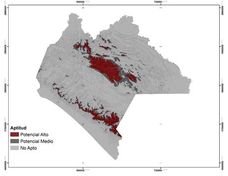
The potential areas for the two species are mainly concentrated in the Sierra Madre region of Chiapas and the Central Highlands (Figures 2 and 3). For P. oocarpa an area of 874 695 ha was delimited, with a high potential for the establishment of UPGF. This species of wide distribution is located at altitudes of 300 to 3 000 m, in poor soils and temperatures between 3 and 35 °C (Eguiluz, 1982; Perry, 1991). For P. pseudostrobus the area was 478 493 ha; for this species, its range of altitudinal distribution is more restricted, from 1 600 to 3 200 m and it develops under minimum temperatures of -9 °C and maximum of 40 °C (Fierros, 1999). However, the limited surface area predicted by the model is mainly due to the fact that P. oocarpa thrives most successfully at altitudes between 900-2 600 m, minimum temperatures of 12 °C and maximum of 22 °C and at moderate soil depths to deep (Eguiluz, 1982); P. pseudostrobus is favored at altitudes of 1 500 to 2 400 m and with temperatures of 14 to 20 °C (Fierros, 1999).

Aptitud = Category; Potencial alto = High potential; Potencial medio = Medium potential; No apto = Not suitable.
Figure 2 Potential areas for the establishment of Forest Germplasm Production Areas and distribution of Pinus oocarpa Schiede ex Schltdl. in Chiapas State.
Aptitud = Category; Potencial alto = High potential; Potencial medio = Medium potential; No apto = Not suitable.
Figure 3 Potential areas for the establishment of Forest Germplasm Production Areas and distribution of Pinus pseudostrobus Lindl. in Chiapas State.
Regarding the variables used (Table 2), altitude was the one that contributed the greatest percentage to the training of the model of both species, this agrees with Schumann et al. (2016) who, when modeling the distribution of 14 species, altitude, turned out to be the most important variable for 11 of them. In other studies with different Pinus species, a positive correlation has been found between altitude and different morphological variables (Sáenz-Romero et al., 2006; Sáenz-Romero et al., 2012; Viveros et al., 2013), so it is expected that this variable contributes in an important with information for both models.
Table 2 Percentage contribution of the variables to the training of the models.
| Variable | Contribution | |
|---|---|---|
| P. oocarpa (%) | P. pseudostrobus (%) | |
| Alt | 84.5 | 97.3 |
| Bio2 | 6.9 | 0 |
| Bio14 | 6.2 | - |
| Eda | - | 0.3 |
| pH | - | 2.4 |
| NDVI | 0.6 | - |
| pp | 1.8 | - |
| tex | - | 0 |
Soil pH influences the availability of most nutrients (Alcántar and Trejo, 2010); however, it is a variable scarcely used in ecological niche modeling. However, for P. pseudostrobus, the pH was incorporated in the modeling, since, in general, it restricts its distribution to soils with a predominantly acidic tendency, with values between 4.5 and 6.5 (Rueda et al., 2006; Eguiluz, 1982), which coincides with the distribution limitations of other coniferous species (Pérez et al., 2014).
Although altitude, temperature, precipitation and type of climate are variables frequently considered in the modeling of the potential distribution of species (Schumann et al., 2016; Qin et al., 2017), in this work only Bio2, Bio14 and pp were used, since these three had a low weight in the construction of the model, due to the high correlation between them (García, 2004; Fries et al., 2012).
The particular route followed by MaxEnt to obtain the optimal solution of the model, results in different results, since a different algorithm could obtain the same solution through a different route, which would lead to different percentage contribution values (Phillips et al., 2006). In this particular case, MaxEnt considered altitude to be more important compared to the rest of the variables used for modeling.
When comparing the results of Table 2, the above is confirmed, since it is observed that altitude alone has a relevant weight in the presence or absence of the two species (> 80 %). This is akin to that recorded by Cruz et al. (2014), with the understanding that said variable has a high percentage (> 85 %) of participation in the model of three forest species. For P. oocarpa, Bio2 and Bio14 showed significant participation in the model, which is similar for Catopheria chiapensis A. Gray ex Benth., Quercus martinezii H. Mull., Telanthopora grandifolia (Less.) H. Rob. & Brettell and Viburnum acutifolium G. Bentham.
The NDVI revealed to be a variable with little percentage contribution to the model. This behavior is attributable to the fact that this vegetation index reflects greenness levels of the vegetation, in this context, the high NDVI values for the study area were obtained from pasture, secondary vegetation of pine-oak forest, medium forest, forests of pine-oak and high evergreen forest. Another disadvantage of this index is saturation with leaf area index values greater than 2 (Huete et al., 1999; Ruiz-Huanca et al., 2005), which is why its use is recommended in arid and semi-arid areas where Schumann et al. (2016) reported good response of this variable when modeling the distribution of species in these ecosystems.
The texture of the soil was the least relevant variable, which is attributable to the level of description of the information contained in the digital cartography used, since it classifies the texture into coarse, medium and fine particles. Fierros et al. (1999) argue that P. pseudostrobus can be established in soils with sandy loam, loam-clay-sandy, clay and clay-sandy soils, while P. oocarpa, in soils with sandy texture, sandy-loamy, sandy-clayey with good drainage (Eguiluz, 1982); this confirms that both species are distributed indistinctly in soils with fine to coarse textures.
The results of the model and the field trips allowed the establishment and registration of two Forest Germplasm Production Units: the UPGF Juznajab (N-07-019-JUZ-001/17) with the two species of interest, and the UPGF Coapilla (N- 07-018-COA-002/17) with P. oocarpa (Figure 4).
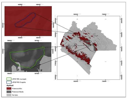
Aptitud = Category; Potencial alto = High potential; Potencial medio = Medium potential; No apto = Not suitable.
Figure 4 Location of the UPGF Coapilla and Juznajab in Chiapas State.
In Juznajab, 2 % of the area was classified as not suitable for P. oocarpa and 98 % was in the medium potential category; for P. pseudostrobus 100 % of the area was cataloged with high potential, which agrees with the conditions observed in the field, which is attributable to the current state of the vegetation as it is an area under forest management with an average cup coverage of 58 %. Likewise, it was confirmed that the precipitation present in this site (1 350 mm) is lower than the optimum required by the species.
Conclusions
The results of the model supported the location of areas suitable for the establishment of UPGF, decreasing the times and costs in the search for areas with optimal conditions. In addition, it is suggested that, in order to generate reliable models at the variety level, it is vital to have a large number of points of presence that correspond specifically to the variety of interest. In the same way it is required to characterize in detail the edaphic conditions and spatially represent the information at a higher spatial resolution than those used in this work.
Acknowledgements
To the Centro de Investigación Regional Pacífico Sur (CIRPAS) of the Instituto Nacional de Investigaciones Forestales, Agrícolas y Pecuarias (INIFAP), for the institutional support provided to accomplish this project. To Eng. Eduardo Rodríguez Chávez and to the Universidad Agraria Antonio Narro for their contribution with the help of the following students: Leonardo C. Cruz Velázquez, Luis A. Natar en Aguilar, David Velasco Reyes, Manuel Pérez Pérez and Francisco A. Chávez Ángel.
REFERENCES
Alba L. J., A. Aparicio R., F. H. Zitácuaro C. y E. O. Ramírez G. 2005. Establecimiento de un ensayo de progenie de Pinus oaxacana Minrov en los Molinos, Municipio de Perote, Veracruz. Foresta Veracruzana 7(2): 33-36. [ Links ]
Alcántar G., G. y L. I. Trejo T. (Coords.) 2010. Nutrición de cultivos. Colegio de Posgraduados, Mundi-Prensa. México, D. F., México. 454 p. [ Links ]
Araujo, M. B. and A. Guisan. 2006. Five (or so) challenges for species distribution modeling. Journal of Biogeography 33(10):1677-1688. [ Links ]
Chávez, P. S. 1996. Image based atmospheric corrections. Revisted and improved. Photogrammetric Engineering and Remote Sensing 2 (9): 1025-1036. [ Links ]
Comisión Nacional Forestal (Conafor). 2014. Informe final de resultados del monitoreo y evaluación complementaria de los apoyos de reforestación y suelos 2012. Universidad Autónoma Chapingo. Texcoco, Edo. de Méx., México. 276 p. [ Links ]
Comisión Nacional para el Conocimiento y Uso de la Biodiversidad (Conabio). 2013. La biodiversidad en Chiapas: Estudio de Estado. Comisión Nacional para el Conocimiento y Uso de la Biodiversidad/Gobierno del Estado de Chiapas. Tuxtla Gutiérrez, Chis., México. 553 p. [ Links ]
Comisión Nacional para el Conocimiento y Uso de la Biodiversidad (Conabio). 2017. Nichos y Áreas de distribución. http://nicho.conabio.gob.mx/la-calibracion-del-modelo (10 de mayo de 2017). [ Links ]
Costa, G. C., C. Nogueira, R. B. Machado and G. R. Colli. 2010. Sampling bias and the use of ecological niche modeling in conservation planning: a field evaluation in a biodiversity hotspot. Biodiversity and Conservation 19(3): 883-899. [ Links ]
Cruz-Cárdenas, G., J. L. Villaseñor, L. López-Mata, E. Martínez-Meyer y E. Ortiz. 2014. Selección de predictores ambientales para el modelado de la distribución de especies en MaxEnt. Revista Chapingo Serie Ciencias Forestales y del Ambiente 20(2):187-201. http://dx.doi.org/10.5154/r.rchscfa.2013.09.034 [ Links ]
Delaney, J. 1999. Geographical information system an introduction. Oxford University Press. Oxford, UK. 194 p. [ Links ]
Dormann, C. F., J. Elith, S. Bacher, C. Buchmann, G. Carl, G. Carré, J. R. García, M., B. Gruber., B. Lafourcade., P. J. Leitao., T. Münkemüller, C. McClean, P. E. Osborne, B. Reuneking, B. Schoröder, A. K. Skidmore, D. Zurell and S. Lautenbach. 2013. Collinearity: a review of methods to deal with it and a simulation study evaluating their performance. Ecography 36(1): 27-46. [ Links ]
Eguiluz P., T. 1982. Clima y distribución del género Pinus en México. Ciencia Forestal 7 (38): 30-44. [ Links ]
Elith, J., C. Graham, R. Anderson, M. Dudík, S. Ferrier, A. Guisan, R. Hijmans, F. Huettmann, J. Leathwick, A. Lehmann, L. Jin, L. G. Lohmann, B. A. Loiselle, G. Manion, C. Moritz, M. Nakamura, Y. Nakazawa, J. M. Overton, A. T. Peterson, S. T. Phillips, K. Richardson, R. Scachetti-Pereira, R. E. Schapire, J. Soberon, S. Williams, M. S. Wisz and N. E. Zimmermann. 2006. Novel methods improve prediction of species’ distributions from occurrence data. Ecography 29(2):129-151. [ Links ]
Enviromental Systems Research (ESRI). 2017. Maps throughout this article were created using Arc-GIS® software. Institute ESRI. Redlands, CA, USA. n/p. [ Links ]
Fierros, A., A. Noguez y E. Velazco. 1999. Establecimiento y manejo de plantaciones forestales comerciales de Pinus oaxacana Mirov. en Chiapas. Paquetes tecnológicos para el establecimiento de plantaciones forestales comerciales en ecosistemas de clima templado - frío y tropicales de México. Semarnap. México, D. F., México. 40 p. [ Links ]
Fernández-Pérez, L., N. Ramírez-Marcial y M. González-Espinosa. 2013. Reforestación con Cupressus lusitanica y su influencia en la diversidad del bosque de pino-encino en Los Altos de Chiapas, México. Botanical Sciences 91(2):207-216. [ Links ]
Fries, A., R. Rollenbeck, T. Naub, T. Peters and J. Bendix. 2012. Near surface air humidity in a megadiverse Andean mountain ecosystem of southern Ecuador and its regionalization. Agricultural and Forest Meteorology 152: 17- 30. [ Links ]
Fuentes D., J., D. Vargas L. y M. Boada J. 2016. Distribución del patrón espacial tipo leopardo en regiones áridas y semiáridas del mundo. Boletín de la Asociación de Geógrafos Españoles 71: 59-72. [ Links ]
García, E. 2004. Modificaciones al sistema de clasificación climática de Köppen. Instituto de Geografía. Universidad Nacional Autónoma de México. 5ª ed. México, D. F., México. 98 p. [ Links ]
Huete, A., C. Justice and W. van Leeuwen. 1999. MODIS Vegetation Index (mod 13) Algorithm Theoretical Basis Document. Ver. 3. https://modis.gsfc.nasa.gov/data/atbd/atbd_mod13.pdf . (15 de abril de 2017). [ Links ]
Ibarra M., J. L., G. Rangel P., F. A. González F., J. de Anda, E. Martínez M. y H. Macías C. 2012. Uso del modelado de nicho ecológico como una herramienta para predecir la distribución potencial de Microcystis sp. (cianobacteria) en la presa hidroeléctrica de Aguamilpa, Nayarit, México. Revista Ambiente & Água - An Interdisciplinary Journal of Applied Science: 7(1), http://dx.doi.org/10.4136/ambi-agua.607. (5 de febrero de 2017). [ Links ]
Instituto Nacional de Estadística y Geografía (Inegi). 2006. Edafología Conjunto de datos vectorial Edafológico escala 1: 250 000 Serie II (Continuo Nacional). http://www.inegi.org.mx/geo/contenidos/recnat/edafologia/vectorial_serieii.aspx (4 de febrero de 2017). [ Links ]
Instituto Nacional de Estadística y Geografía (Inegi). 2008. Climatología Datos vectoriales escala 1:1000000. http://www.inegi.org.mx/geo/contenidos/recnat/clima/infoescala.aspx (4 de febrero de 2017). [ Links ]
Instituto Nacional de Estadística y Geografía (Inegi). 2016. Marco Geoestadístico Nacional. Ver. 6. http://www.inegi.org.mx/geo/contenidos/geoestadistica/m_geoestadistico.aspx (4 de febrero de 2017). [ Links ]
Kearney, M. 2006. Habitat, environment and niche: what are we modelling? Oikos 115(1):186-191. [ Links ]
Kulloli, R. N. and S. Kumar. 2014. Comparison of bioclimatic, NDVI and elevation variables in assessing extent of Commiphora wightii (Arnt.) Bhand. The International Archives of the Photogrammetry, Remote Sensing and Spatial Information Sciences 8: 9-14. [ Links ]
Liu, C., P. M. Berry, T. P. Dawson and R. G. Pearson. 2005. Selecting thresholds of occurrence in the prediction of species distributions. Ecography 28(3): 385-393. [ Links ]
Morales, S. N. 2012. Modelos de distribución de especies: Software Maxent y sus aplicaciones en Conservación. Conservación Ambiental 2 (1): 1-5. [ Links ]
Muñoz F., H. J., J. Muñoz G., H. Hernández A., J. J. García M., V. M. Coria A. y J. Hernández R. 2014. Caracterización dasométrica de tres rodales semilleros de especies del género Pinus en el estado de Guerrero, México. Foresta Veracruzana 16(2): 23-30. [ Links ]
Navarro-Cerrillo, R. M., J. E. Hernández-Bermejo and R. Hernández-Clemente. 2011. Evaluating models to assess the distribution of Buxus balearica in southern Spain. Applied Vegetation Science 14(2): 256-267. [ Links ]
Norris, D. 2014. Model thresholds are more important than presence location type: Understanding the distribution of lowland tapir (Tapirus terrestris) in a continuous Atlantic forest of southeast Brazil. Tropical Conservation Science 7 (3): 529-547. [ Links ]
Pérez M., R., F. Moreno S., A. González H y V. J. Arriola P. 2014. Distribución de Abies religiosa (Kunth) Schltdl. et Cham. y Pinus montezumae Lamb. ante el cambio climático. Revista Mexicana de Ciencias Forestales 5(25): 18-33. [ Links ]
Perosa, M., J. F. Rojas, P. E. Villagra, M. F. Tognelli, R. Carrana y J. A. Álvarez. 2014. Distribución potencial de los bosques de Prosopis fexuosa en la Provincia Biogeográfica del Monte (Argentina). Ecología Austral 24 (2): 238-248. [ Links ]
Perry, J. P. 1991. The Pines of Mexico and Central America. Timber Press. Portland, OR, USA. 234 p. [ Links ]
Phillips, S. J., R. P. Anderson and R. E. Schapire. 2006. Maximum entropy modeling of species geographic distributions. Ecological Modelling 190(3-4): 231-259. [ Links ]
Phillips, S. J. and M. Dudík. 2008. Modeling of species distributions with Maxent: new extensions and a comprehensive evaluation. Ecography 31(2): 161-175. [ Links ]
Plasencia-Vázquez, A. H., G. Escalona-Segura y L. G. Esparza-Olguín. 2014. Modelación de la distribución geográfica potencial de dos especies de psitácidos neotropicales utilizando variables climáticas y topográficas. Acta Zoológica Mexicana 30 (3): 471-490. [ Links ]
Qin, A., B. Liu, Q. Guo, R. W. Bussmann, F. Ma, Z. Jian, G. Xu and S. Pei. 2017. Maxent modeling for predicting impacts of climate change on the potential distribution of Thuja sutchuenensis Franch., an extremely endangered conifer from southwestern China. Global Ecology and Conservation 10: 139-146. [ Links ]
Rueda S., A., J. A. Ruíz C., J. G. Flores G. y E. Talavera Z. 2006. Potencial productivo para 11 especies de pino en Jalisco. Campo Experimental Centro Altos de Jalisco, CIRPAC, INIFAP. Libro Técnico Núm. 1. Guadalajara, Jal., México. 175 p. [ Links ]
Ruiz-Huanca, P., E. Palacios-Vélez, E. Mejía-Saenz, A. Exebio-García, J. L. Oropeza-Mota y M. Bolaños-González. 2005. Estimación temprana del rendimiento de la cebada mediante uso de sensores remotos. Terra Latinoamericana 23 (2):167-174. [ Links ]
Rzedowski, J. 2006. Vegetación de México. 1ª edición digital. Comisión Nacional para el Conocimiento y Uso de la Biodiversidad. México, D. F., México. 504 p. http://www.biodiversidad.gob.mx/publicaciones/librosDig/pdf/VegetacionMx_Cont.pdf (12 de marzo de 2017). [ Links ]
Sáenz-Romero, C., R. R. Guzmán-Reyna and G. E. Rehfeldt. 2006. Altitudinal genetic variation among Pinus oocarpa populations in Michoacán, Mexico Implications for seed zoning, conservation, tree breeding and global warming. Forest Ecology and Management 229: 340-350. [ Links ]
Sáenz-Romero, C., G. R. Rehfeldt, J. C. Soto-Correa, S. Aguilar-Aguilar, V. Zamarripa-Morales and J. López-Upton. 2012. Altitudinal genetic variation among Pinus pseudostrobus populations from Michoacán, México. Two location shadehouse test results. Revista Fitotecnia Mexicana 35(2): 11-120. [ Links ]
Schumann, K., B. M. I. Nacoulma, K. Hahn, S. Traor, A. Thiombiano and Y. Bachmann. 2016. Modeling the distributions of useful woody species in eastern Burkina Faso. Journal of Arid Environments 135: 104-114. DOI: 10.1016/j.jaridenv.2016.08.017. [ Links ]
Secretaría de Economía. 2016. Declaratoria de vigencia de la Norma Mexicana: Establecimiento de unidades productoras y manejo de germoplasma forestal-especificaciones técnicas. NMX-AA-169-SCFI-2016. Diario Oficial de la Federación Diario Oficial de la Federación http://www.dof.gob.mx/nota_detalle.php?codigo=5455455&fecha=03/10/2016ttp://www.dof.gob.mx/nota_detalle.php?codigo=5455455&fecha=03/10/2016 (25 de marzo de 2017). [ Links ]
Servicio Meteorológico Nacional (SMN). 2010. Normales climatológicas por estado. http://smn.conagua.gob.mx/es/informacion-climatologica-ver-estado?estado=chis (4 de enero de 2017). [ Links ]
Vanegas L., M. 2016. Manual de mejores prácticas de restauración de ecosistemas degradados, utilizando para reforestación solo especies nativas en zonas prioritarias. Conafor-Conabio. México, D. F., México. 158 p. [ Links ]
Viveros-Viveros, H., C. Sáenz-Romero, J. López-Upton and J. J. Vargas-Hernández. 2007. Growth and frost damage variation among Pinus pseudostrobus, P. montezumae and P. hartwegii tested in Michoacán, México. Forest Ecology and Management 253(1-3): 81-88. [ Links ]
Viveros-Viveros, H., A. R. Camarillo L., C. Sáenz R. y A. Aparicio R. 2013. Variación altitudinal en caracteres morfológicos de Pinus patula en el estado de Oaxaca (México) y su uso en la zonificación. Bosque 34 (2): 173-179. [ Links ]
Wan, J., C. Wan, J. Yu, S. Nie, S. Han, J. Liu, Y. Zu and Q. Wang. 2015. Developing conservation strategies for Pinus koraiensis and Eleutherococcus senticosus by using model-based geographic distributions. Journal of forestry Research 27 (2): 389-400. [ Links ]
Received: May 31, 2017; Accepted: May 17, 2018
 Este es un artículo publicado en acceso abierto bajo una licencia Creative Commons
