


Servicios Personalizados
Revista
Articulo
 texto en
  Inglés (pdf)
 Artículo en XML
 Referencias del artículo
 Enviar artículo por email
Indicadores
-
 Citado por SciELO
 -
 Accesos
Links relacionados
-
 Similares en
SciELO
Similares en
SciELO
Compartir

 Permalink
Revista mexicana de ciencias forestales
versión impresa ISSN 2007-1132
Rev. mex. de cienc. forestales vol.9 no.47 México may./jun. 2018
https://doi.org/10.29298/rmcf.v9i47.160
Articles
Environmental variables affecting the density of ten forest species in the Northern Sierra of Oaxaca
1Maestría en Ciencias en Conservación de los Recursos Forestales, Universidad de la Sierra de Juárez. México.
2División de estudios de Posgrado, Instituto de Estudios Ambientales, Universidad de la Sierra de Juárez. México.
The characterization of the environmental conditions of forest species is important because it allows knowing part of their habitat; this information is useful for making decisions for an integral use of forests, including preventive measures that counteract habitat degradation or the risk of extinction of the plants. The main objective of this study was to identify the environmental variables that significantly affect the abundance of ten tree species growing in the temperate forests of Santiago Comaltepec, north of Oaxaca. Three analysis methods were used for this purpose: 1) principal component analysis, 2) non-parametric correlation coefficients, and 3) generalized linear models. A total of 23 climatic and physiographic variables were used: mainly records of average, minimum and maximum temperatures; rainfall during the summer, spring and winter, and rainfall during of the highest plant activity, as well as other attributes of each sampling plot including the slope, exposure and altitude. All the variables studied showed a significant correlation (p<0.001) with at least three species, several of them with correlation coefficients greater than 0.90. Of the ten species studied, three showed high sensitivity to temperature variables, mainly the minimum temperature, temperatures above 5 °C, and the aridity index; and three species showed high evidence of sensitivity to the precipitations registered in spring, in summer and in winter, and to the April-September precipitations.
Keywords: Abundance; multivariate analysis; temperate forest; non-parametric correlation; generalized additive models; climatic niche
Caracterizar las condiciones ambientales en las que se desarrollan las especies forestales es importante, porque permite conocer parte de su hábitat; información útil para tomar decisiones encaminadas a un aprovechamiento integral de los bosques, que incluya medidas preventivas que contrarresten su degradación o su extinción. El objetivo de este estudio fue identificar las variables ambientales que afectan significativamente la abundancia de 10 especies arbóreas que crecen en los bosques templados de Santiago Comaltepec, al norte de Oaxaca, México. Para ello, se utilizaron tres métodos de análisis: 1) componentes principales, 2) coeficientes de correlación no paramétrica, y 3) modelos lineales generalizados. Se evaluaron un total de 23 variables medioambientales, principalmente, registros de temperaturas mínimas y máximas; precipitaciones en el verano, en invierno y en primavera; así como atributos fisiográficos que incluyeron la pendiente, la exposición y la altitud. Todas mostraron una correlación significativa (p<0.001) con al menos tres especies, varias con coeficientes de correlación superior a 0.90. Se identificaron tres taxa que son más sensibles a las variables de temperatura, en particular, a la temperatura mínima, la superior a 5 °C, y al índice de aridez; otras tres que parecen tener mayor sensibilidad a la cantidad de lluvia registrada en la primavera, en el verano, en el invierno y en las precipitaciones de abril a septiembre.
Palabras clave: Abundancia; análisis multivariado; bosque templado; correlación no paramétrica; modelos lineales generalizados; nicho climático
Introduction
The characterization of the habitat of forest species is important for understanding their geographical distribution, abundance or presence at a given location. This information is helpful for making appropriate decisions when implementing conservation, integral management or preventive actions to counteract the degradation of the habitat or the extinction of the plants (Anderson et al., 2003). Some of the most widely used variables are climatic, physiographic and edaphological (Guisan and Zimmermann, 2000; Arundel, 2004; González-Espinosa et al., 2004) primarily, temperature, precipitation, altitude, slope and geographical orientation (Pliscoff and Fuentes-Castillo, 2001; Antúnez et al., 2017b). Different methods are used for studying the relationship between these factors and the distribution and abundance of plants, including the correlative mathematic tools. Examples of these are the correlation analyses (Bravo et al., 2008; Bravo-Iglesias, 2010), utilized in the forest area for identifying relevant population parameters or environmental factors that are important for the distribution and abundance (Bravo-Iglesias, 2010; Martínez-Antúnez et al., 2013).
Multivariate analyses, in their various modalities, often applied to reduce the number of variables (Buira, 2017; Guisan et al., 1999); multiple regression analysis, used to detect the factors with greatest influence on the abundance of plants (Martínez-Antúnez et al., 2015), and generalized linear models (Guisan et al., 1999). These three methods have yielded satisfactory results in similar studies, by identifying, out of a set of variables, those that significantly affect a variable of interest (Arredondo-Figueroa et al., 1984; Guisan et al., 1999); this, in turn, makes it possible to distinguish high-impact covariables that may condition those localities where the forest species of interest are distributed (Araújo and Guisan, 2006; Antúnez et al., 2017a).
On the other hand, 95 % of all forestry activities are concentrated in temperate forests, primarily in pine, pine-oak or oak-pine forests (Masera et al., 1997). In this regard, the Northern Sierra of Oaxaca is one of the regions of southeastern Mexico where forestry activity has increased in the last decades, in keeping with an equally growing regional market (Castellanos-Bolaños et al., 2008). Pinus patula Schiede ex Schltdl. et Cham and Pinus pseudostrobus Lindl. (currently known as Pinus oaxacana Mirov. by forest managers) stand out for their commercial interest (Antúnez et al., 2017a), despite the prevalence of broadleaf species, particularly of the genus Quercus, for which, nevertheless, there is no stable or safe market (Alfonso-Corrado et al., 2014).
The objective of this study was to identify the environmental variables that significantly affect the density of the ten most prevalent native forest species in Santiago Comaltepec, a locality of the Northern Sierra of Oaxaca. Three analysis methods were used for this purpose: non-parametric correlation coefficient, principal component analysis and generalized linear models.
Materials and Methods
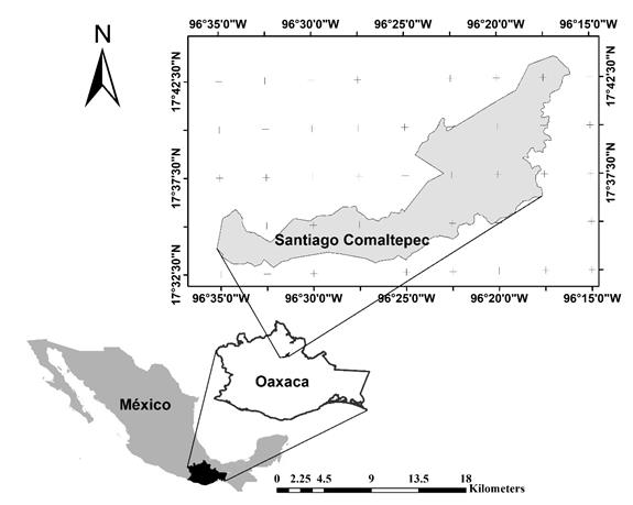
The research was carried out in the forests of Santiago Comaltepec, located in the Northern Sierra of Oaxaca, in southeastern Mexico, between the coordinates 17°34’32’’ N and 96°29’45” W, at an altitude of 1 924 to 3 000 masl, on a surface area of approximately 26.5 km2 (Figure 1). The predominant types in the area are humid temperate, humid warm and humid semi-warm, with summer rains and a mean annual temperature of 9.5 °C and 16.2 °C. The most common types are: Acrisol, Luvisol and Cambisol (Conabio, 1999; Inegi, 2012).
The ten most abundant tree species that turned out to be the most representative of Santiago Comaltepec and adjoining localities (San Pedro Yólox, San Juan Bautista Valle Nacional, Ayotzintepec, Ixtlán de Juárez, San Pablo Macuiltianguis and San Juan Quiotepec) were: Alnus acuminata Kunth, Alnus firmifolia Fern, Pinus ayacahuite C. Ehrenb. ex Schltdl., Pinus hartwegii Lindl., Pinus teocote Schiede ex Schltdl. et Cham., Quercus crassifolia Bonpl., Quercus laurina Bonpl., Quercus rugosa Née, Arbutus xalapensis var. pubescens Benth. and Prunus serotina Ehrh. subsp. capuli (Cav. ex Spreng.) McVaugh.
The data were collected in 433 privately-owned 1 000 m2 round plots, systematically distributed according to such conditions as vegetation type, relief and quality of the season. This study utilized the same sampling design as the owners and forest managers in order to quantify the volumetric stock of extractable lumber. The tree species occurring in each plot were identified; individuals with a diameter equal to or above 7.5 cm (at 1.3 m above the ground) were counted, as the diameter was considered to be an indicator of both survival and growth (Sáenz et al., 2010).
The density (number of individuals per plot) was used as indicator of abundance (Martínez-Antúnez et al., 2013; Antúnez et al., 2017a). A total of 23 environmental variables were included; their acronyms and descriptive statistics are shown in Table 1. The climate records were obtained using a modeler of the Forest Service, Department of Agriculture of the United States, which estimated accurate values for each sampling unit based on a climate record of little more than 6 000 weather stations in Mexico, the south of the United States, Guatemala, Belize and Cuba, from 1961 to 1990 (Crookston et al., 2008; Sáenz-Romero et al., 2010). The slope and exposure were measured in field with a SuntoTM clinometer, and the altitude was registered using a GarminTM Global Positioning System (GPS) receiver.
Table 1 Acronyms and descriptive statistics of the variables used to characterize the abundance of 10 forest species.
| Variables | Average | Typical deviation | Minimum | Maximum |
|---|---|---|---|---|
| MAT | 11.57 | 1.42 | 9.5 | 16.2 |
| MAP | 2092.81 | 463.69 | 1307 | 3063 |
| GSP | 1548.52 | 319.70 | 1014 | 2220 |
| MTCM | 9.72 | 1.34 | 7.6 | 13.8 |
| MMIN | 4.65 | 1.03 | 2.9 | 7.6 |
| MTWM | 13.88 | 1.48 | 12 | 18.9 |
| MMAX | 19.80 | 1.74 | 17.4 | 25.7 |
| FFP | 274.18 | 45.14 | 194 | 364 |
| SDAY | 41.99 | 22.32 | 1 | 81 |
| FDAY | 326.09 | 18.39 | 296 | 364 |
| DD5 | 2408.56 | 497.14 | 1699 | 4056 |
| GSDD5 | 2022.47 | 663.85 | 1098 | 4047 |
| D100 | 21.42 | 4.89 | 11 | 32 |
| MMINDD0 | 38.06 | 25.31 | 0 | 101 |
| SMRPB | 2.31 | 0.10 | 2.06 | 2.5 |
| SMRSPRPB | 5.55 | 0.14 | 5 | 5.89 |
| SPRP | 124.37 | 24.67 | 83 | 174 |
| SMRP | 693.61 | 152.89 | 444 | 1019 |
| WINP | 285.28 | 75.13 | 151 | 441 |
| AI | 0.0 | 0.0 | 0.0 | 0.0 |
| MSEP | 38.84 | 22.15 | 10 | 95 |
| EXP | 5.79 | 2.58 | 1 | 9 |
| HASL | 2596.25 | 257.15 | 1924 | 3002 |
MAT = Mean annual temperature (°C); MAP = Mean annual precipitation (mm); GSP = Mean precipitation in the growing season (mm);MTCM = Mean temperature in the coldest month (January) (°C); MMIN = Mean minimum temperature in the coldest month (°C); MTWM = Mean temperature in the warmest month (June); MMAX = Mean maximum temperature in the warmest month (°C); FFP = Length of the frost-free period (days); SDAY = Day of the year of the last spring frost (day); FDAY = Julian date of the last freezing date of spring (day); DD5 = Degree-days >5º C (degrees-days); GSDD5 = Degree-days >5ºC accumulating within the frost-free period (degrees-days); D100 = Julian date the sum of degree-days >5º C reaches 100 (degrees-days); MMINDD0 = Minimum degree-days < 0 °C (degrees-days); SMRPB = Summer precipitation balance (July+August+September/April+May+June) (mm); SMRSPRPB = Summer/spring precipitation balance (July+August/April+May) (mm); SPRP = Spring precipitation (mm); SMRP = Summer precipitation (mm); WINP = Winter precipitation (mm); IA = Aridity index; PEN = Mean slope of each plot (%); EXP = (1= Zenithal, 2=Northern, 3=Northeastern, 4=Eastern, 5=Southeastern, 6=Southern, 7=Southwestern, 8=Western, and 8=Northwestern) exposure, and HASL = Height above the sea level (m).
Data analysis
In order to identify the variables significantly affecting the abundance of each of the studied species, the following analyses were used: 1) parametric coefficient of correlation using the Bootstrap technique (James and McCulloch, 1990; Sideridis and Simos, 2010) when detecting data that do not follow a normal distribution; 2) principal component analysis (PCA) in order to reduce the number of variables the spatial auto-correlation of the data was considered whenever possible, and 3) generalized lineal models (GLM) (Nelder and Wedderburn, 1972) in order to identify a causal relationship. The third was used to assess the individual contribution of each covariate, according to its parameter and significance level (p<0.05), as well as the values of the Akaike information criterion (AIC); the global deviance (DE) and the Hosmer-Lemeshow test values (Hosmer and Lemeshow, 2000). All the analyses were carried out using the R (R Core Team, 2017) software.
Results and Discussion
The principal component analysis revealed that the variables that account for the largest percentage of variability of the abundance of Alnus acuminata, A. firmifolia, Pinus ayacahuite, P.teocote, Quercus crassifolia, Q. rugosa and Arbutus xalapensis were the temperatures above 5 °C (GSDD5 and DD5), the mean annual precipitation (MAP), the height above the sea level (HASL) and the April-September precipitation, with 96.5 % variability. This precipitation period is important for the plants because it coincides with the increase in the vegetative activity (Sáenz-Romero et al., 2010; Martínez-Antúnez et al., 2013; Antúnez et al., 2017b). The rest of the variables accounted only for 3.4 % of the variability of the data (Figures 2A and 2B). For the abundance of P. hartwegii, Q. laurina and Prunus serotina, the most relevant variables were GSDD5, MAP, DD5, GSP and HASL (97.73 %). The rest accounted only for 2.13 % of the variability (Figure 2C and 2D).
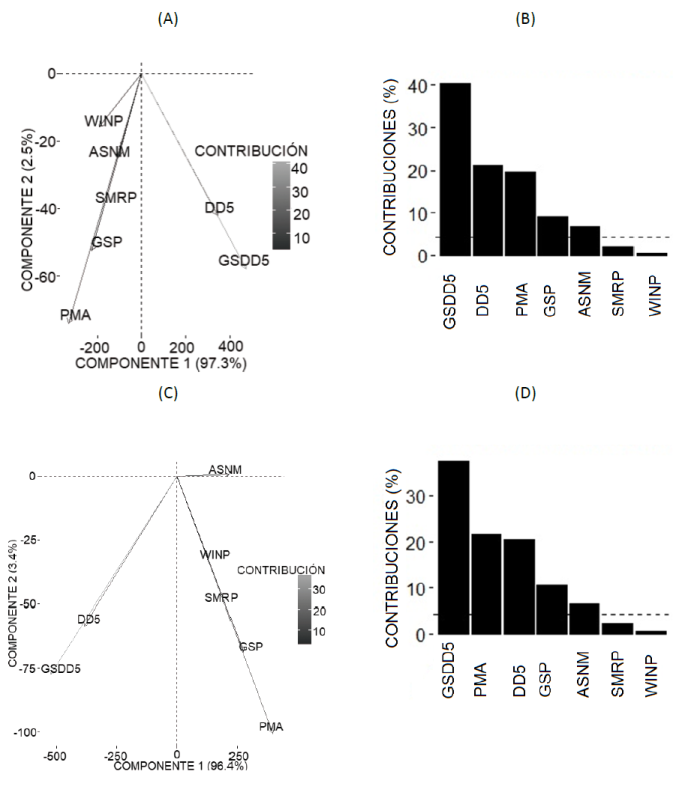
Contribución = Contribution; Conponente = Component
The seven most important variables for Pinus ayacahuite (B) and the seven most important for Pinus hartwegii, Pinus serotina and Quercus laurina (D). GSDD5 = Degree-days > 5 °C accumulating within the frost-free period; DD5 = Degree-days > 5 °C; PMA = Mean annual precipitation (mm) (MAP),GSP = April to September precipitation; HASL = Height above the sea level; SMRP = Summer precipitation; WINP = Winter precipitation.
Figure 2 Variables that most contributed to explain the variability of Pinus ayacahuite C. Ehrenb. ex Schltdl. (A) and of P. harwegii Lindl. (C), according to the principal component analyses.
Each species is affected by different variables (tables 2 and 3); for example, the mean annual precipitation and the April-September precipitation exhibited high coefficients, with an abundance of Q. laurina (0.99-0.99), P. ayacahuite (0.85-0.86) and P. hartwegii (0.99-0.99), but not with A. acuminata or A. xalapensis, which had low or null correlations (0.09-0.10) (0.001) (Table 2). Likewise, the abundance of Q. laurina, P. ayacahuite and P. hartwegii were significantly correlated (0.85 to 0.99) with the precipitations during spring, summer and winter (SPRP, SMRP and WINP), in agreement with authors like Jabro et al. (2010), Wittmer et al. (2010) and Meng et al. (2011), who highlight the importance of the intensity and the magnitude of the rains, as well as of the precipitation period, on the distribution of the plants.
Table 2 Correlation coefficients between the abundance of the ten studied species and each of the environmental variables.
| Variables | Species | |||||||||
|---|---|---|---|---|---|---|---|---|---|---|
| Arb. xal. | Aln. acu. | Que. rug. | Que. cras | Pru. ser. | Aln. fir. | Pin. aya. | Pin. har. | Pin. teo. | Que. lau. | |
| MAT | 0.96 | 0.83 | 0.81 | 0.71 | 0.68 | 0.54 | 0.21 | <0.05 | 0.46 | <0.05 |
| MAP | <0.05 | 0.09 | 0.28 | 0.23 | 0.34 | 0.29 | 0.86 | 0.99 | 0.59 | 0.99 |
| GSP | <0.05 | 0.10 | 0.28 | 0.23 | 0.34 | 0.29 | 0.85 | 0.99 | 0.58 | 0.99 |
| MTCM | 0.97 | 0.85 | 0.80 | 0.71 | 0.67 | 0.56 | 0.23 | <0.05 | 0.45 | <0.05 |
| MMIN | 0.97 | 0.84 | 0.80 | 0.72 | 0.69 | 0.58 | 0.21 | <0.05 | 0.48 | <0.05 |
| MTWM | 0.94 | 0.84 | 0.83 | 0.69 | 0.70 | 0.50 | 0.23 | <0.05 | 0.45 | <0.05 |
| MMAX | 0.96 | 0.84 | 0.82 | 0.70 | 0.70 | 0.52 | 0.21 | <0.05 | 0.46 | <0.05 |
| SDAY | <0.05 | 0.10 | 0.20 | 0.21 | 0.28 | 0.51 | 0.85 | 0.99 | 0.63 | 0.99 |
| FDAY | 0.99 | 0.89 | 0.85 | 0.77 | 0.69 | 0.56 | 0.19 | <0.05 | 0.42 | <0.05 |
| FFP | 0.99 | 0.90 | 0.81 | 0.74 | 0.70 | 0.51 | 0.17 | <0.05 | 0.44 | <0.05 |
| DD5 | 0.96 | 0.84 | 0.81 | 0.69 | 0.69 | 0.54 | 0.22 | <0.05 | 0.47 | <0.05 |
| GSDD5 | 0.96 | 0.86 | 0.82 | 0.72 | 0.71 | 0.52 | 0.21 | <0.05 | 0.45 | <0.05 |
| D100 | <0.05 | 0.14 | 0.28 | 0.20 | 0.33 | 0.42 | 0.81 | 0.99 | 0.59 | 0.99 |
| MMINDD0 | <0.05 | 0.13 | 0.35 | 0.20 | 0.36 | 0.26 | 0.80 | 0.99 | 0.64 | 0.99 |
| SMRPB | <0.05 | 0.06 | 0.20 | 0.22 | 0.33 | 0.38 | 0.85 | 0.99 | 0.66 | 0.99 |
| SMRSPRPB | <0.05 | 0.42 | 0.26 | 0.51 | 0.58 | 0.12 | 0.52 | 0.99 | 0.52 | 0.88 |
| SPRP | <0.05 | 0.07 | 0.27 | 0.21 | 0.34 | 0.30 | 0.86 | 0.99 | 0.57 | 0.99 |
| SMRP | <0.05 | 0.10 | 0.28 | 0.23 | 0.33 | 0.28 | 0.85 | 0.99 | 0.58 | 0.99 |
| WINP | <0.05 | 0.08 | 0.27 | 0.20 | 0.33 | 0.32 | 0.86 | 0.99 | 0.62 | 0.99 |
| AI | 0.99 | 0.91 | 0.27 | 0.72 | 0.68 | 0.62 | 0.15 | <0.05 | 0.46 | 0.99 |
| MSEP | 0.97 | 0.12 | 0.44 | 0.47 | 0.18 | 0.85 | 0.96 | <0.05 | 0.92 | 0.57 |
| EXP | 0.37 | 0.24 | 0.60 | 0.33 | 0.62 | 0.81 | 0.99 | 0.46 | 0.63 | 0.68 |
| HASL | <0.05 | 0.16 | 0.17 | 0.29 | 0.28 | 0.36 | 0.83 | 0.99 | 0.50 | 0.99 |
Arb. xal.= Arbutus xalapensis; Aln. acu. = Alnus acuminata; Que. rug.= Quercus rugosa; Que. cras. = Quercus crassifolia; Pru. ser. = Prunus serotina; Aln. fir. = Alnus firmifolia; Pin. aya. = Pinus ayacahuite; Pin. har. = Pinus hartwegii; Pin. teo. = Pinus teocote; Que. lau. = Quercus laurina; MAT = Mean annual temperature; MAP = Mean annual precipitation; GSP = April-September precipitation; MTCM =Mean temperature in the coldest month; MMIN = Mean minimum temperature in the coldest month; MTWM = Mean temperature in the warmest month; MMAX = Maximum mean temperature in the warmest month; FFP = Length of frost-free period; SDAY = Julian date of the last spring freeze; FDAY = Day of the year of the last frost; DD5 = Degree-days > 5 °C; GSDD5 = Degree-days > 5 °C accumulating within the frost-free period; D100 = Julian date that the sum of degree-days > 5 °C reaches 100; MMINDD0 = Minimum degree-days < 0 °C; SMRPB = Summer precipitation balance; SMRSPRPB = Summer/spring precipitation balance; SPRP = Spring precipitation; SMRP = Summer precipitation; WINP = Winter precipitation; AI = Aridity index; MSEP = Mean site slope; EXP = Average site exposure in relation to the cardinal directions (1=Zenithal, 2=Northern; 3=Northeastern; 4=Eastern, 5=Southeastern, 6=Southern, 7=Southwestern, 8=Western and 9=Northwestern); HASL = Height above sea level. The correlation coefficients highlighted in gray were not significant (P<0.05).
Table 3 Variables significantly affecting the abundance of the studied species according to the generalized additive models (p<0.05).
| Species | VAR | PAR | SE | Z | P-value | DE | AIC | H-L (P-value) |
|---|---|---|---|---|---|---|---|---|
| Alnus acuminata | MAT | -32.04 | 12.03 | -2.66 | 0.007** | 2.06 | 143.5 | 0.452 |
| MAP | -1.49 | 0.72 | -2.06 | 0.039* | ||||
| MSEP | -0.04 | 0.02 | -2.38 | 0.0170* | ||||
| Pinus ayacahuite | INTERCEPTO | 1431.00 | 532.40 | 2.688 | 0.007** | 1.41 | 162.8 | 0.830 |
| MMAX | -17.92 | 8.61 | -2.08 | 0.037* | ||||
| SMRPB | -182.10 | 80.29 | -2.26 | 0.023* | ||||
| HASL | -0.23 | 0.08 | -2.93 | 0.003** | ||||
| MSEP | 0.02 | 0.01 | 2.52 | 0.011* | ||||
| Quercus laurina | MMINDD0 | -0.39 | 0.19 | -2.03 | 0.041* | 1.25 | 464.3 | 0.049 |
| AI | 56690.00 | 25810.00 | 2.19 | 0.028* | ||||
| MSEP | 0.01 | 0.01 | 2.20 | 0.027* | ||||
| Pinus hartwegii | MTCM | -25.93 | 9.67 | -2.68 | 0.007** | 1.79 | 178.5 | 0.985 |
| FFP | 0.44 | 0.15 | 2.95 | 0.003** | ||||
| SMRPB | -125.30 | 62.83 | -1.99 | 0.046* | ||||
| MSEP | 0.04 | 0.01 | 2.97 | 0.002** | ||||
| HASL | -0.11 | 0.05 | -2.35 | 0.018* | ||||
| Quercus rugosa | MMIN | 12.03 | 5.70 | 2.10 | 0.035* | 1.53 | 345.6 | 0.080 |
| MMINDD0 | 0.56 | 0.25 | 2.22 | 0.025* | ||||
| MSEP | 0.02 | 0.01 | 2.35 | 0.018* | ||||
| Pinus teocote | MAT | -21.87 | 9.51 | -2.29 | 0.022* | 2.03 | 157.9 | 0.767 |
| FFP | -0.23 | 0.11 | -2.13 | 0.033* | ||||
| MSEP | 0.04 | 0.01 | 2.79 | 0.005** | ||||
| HASL | 0.15 | 0.06 | 2.41 | 0.015* | ||||
| Arbutus xalapensis | MSEP | 0.02 | 0.01 | 2.45 | 0.013* | 1.66 | 363 | 0.005* |
VAR =Variables; PAR = Parameters; MAT =Mean annual temperature; MAP =Mean annual precipitation; MTCM = Mean temperature in the coldest month; MMIN = Mean minimum temperature in the coldest month; MMAX = Mean maximum temperature in the warmest month; FFP = Length of frost-free period; DD5 = Degree-days > 5 °C; MMINDD0 = Minimum degree-days < 0 °C; SMRPB = Summer precipitation balance; AI = Aridity index; MSEP = Slope; HASL = Height above the sea level; DE = Global deviance; AIC = Akaike information criterion;* and *** = Significant values at a significance level of 0.05 and 0.001, respectively; SE = Standard error; H-L = Hosmer-Lemeshow test.
Furthermore, the slope and the exposure had high levels of association with certain species like Arbutus xalapensis (0.97), Alnus firmifolia (0.85-0.81), P. ayacahuite (0.96-0.99) and P. teocote (0.92); conversely, low values were observed with A. acuminata (0.12), P. serotina (0.18) and P. hartwegii (0.01-0.46). As for the variables that exhibited high, significant coefficients, several did not contribute significantly to the generalized models. This suggests a poor causal relationship (Table 3), given that the incidence of most of the variables may have an indirect impact, enhancing or inhibiting those variables that may have a direct effect (Antúnez et al., 2017b). Variables with low associations indicate a limited linear relationship. For example, physiographic variables exhibited low, non-significant coefficients for most species, consistently with the findings of Martínez-Antúnez et al. (2013), who cite very low association coefficients (<0.70) between the physiographic variables exposure and slope and the abundance of the species. In this study, only 35 out of 72 taxa exhibited significant coefficients (p<0.05). However, in other studies, physiographic variables like altitude or terrain slope play an important role in the distribution of pine and oak taxa, as in the case of Q. glaucescens Bonpl., Q. elliptica Née, Q. corrugata Hook., Q. ocoteifolia Liebm. and Q. macdougallii Martínez in Chinantla (Poulos and Camp, 2005; Meave et al., 2006), or exposure, as in the case of Quercus potosina Trel. and Juniperus deppeana Steud. in Sierra Fría, Aguascalientes, where the northern exposure proved adequate for both species (Díaz et al., 2012).
The generalized models indicated that at least one variable has a significant effect on the abundance of seven species (p<0.05), which implies a potential causal relationship between these variables and the abundance of the taxa (Table 3). Thus, the mean annual temperature, the mean annual precipitation and the terrain slope were the most important variables for Alnus acuminata (Table 3). Slope was the only variable with significant effects on the seven species (Table 3). There were few variables that had a limited linear relationship with the abundance of forest species in the study area; this was pointed out also by Antúnez et al. (2017a), who ascribed this fact to the rough, uneven topography of the study area, resulting in different microclimates even within distances of 200 m (Antúnez et al., 2017a).
The results of the principal components analysis showed that the most important variables for the abundance of most species is temperature above 5 °C; however, it is uncertain whether this relationship is causal or merely a correlation. Several results of this analysis agreed with those yielded by the correlation analysis, particularly in regard to temperature above five degrees, with significant coefficients for the abundance of A. xalapensis, A. acuminata and Q. rugosa, whose values ranged between 0.81 and 0.96 (Table 2).
The volume and intensity of the rainfall is one of the key factors in the distribution and abundance of forest vegetation; for example, according to Álvarez-Moctezuma et al. (1999), the precipitation and altitude variables are the most important for the distribution of Quercus peduncularis Née, Q. polymorpha Schltdl. et Cham, Q. rugosa, Q. sebifera Trel. and Q. segoviensis Liebm. in the Central Plateau of Chiapas, Mexico. In the present study, the mean annual precipitation and the April-September precipitation accumulated mean were significantly correlated to P. ayacahuite (0.86-0.85), P. hartwegii (0.99-0.99) and Q. laurina (0.99-0.99) (Table 2), which suggests that these three would be the taxa most severely affected by a modification of the above variables (Sáenz-Romero et al., 2010;Antúnez et al., 2017a).
As for precipitation, results suggest that the April-September precipitations have a stronger impact than the mean annual precipitation on the abundance of P. ayacahuite, P. hartwegii and Q. laurina, with coefficients above 0.85 (Table 1). The influence of precipitation in various seasons (spring, summer, winter or April-September) on the abundance of certain conifers has been observed to be even stronger than the annual mean or the temperature variables (Martínez-Antúnez et al., 2013; Antúnez et al., 2017a). Conversely, the abundance of Abies durangensis Martínez, Quercus resinosa Liebm., Q. acutifolia Née, Q. urbanii Trel. and P. leiophylla Schiede ex Schltdl. et Cham is highly associated to the April-September precipitation, as well as to the mean annual precipitation (Martínez-Antúnez et al., 2013). Other species like Quercus peduncularis, Q. polymorpha, Q. rugosa, Q. sebifera and Q. segoviensis appear to respond to the variations in precipitation, although modified by the altitude (Álvarez-Moctezuma et al., 1999). As for frosts (SDAY, FDAY and FFP), high correlations were observed with the abundance of Q. laurina, P. ayacahuite and P. hartwegii, which exhibited correlation coefficients ranging from 0.85 to 0.99. In this sense, Martínez-Antúnez et al. (2013) document similar values with covariance coefficients above 0.90 for Pseudotsuga menziesii (Mirb.) Franco and Pinus arizonica Engelm. in northwestern Mexico.
In general, the results obtained using the three analysis methods are an important contribution to the characterization of the habitat of the most abundant species of the study area, since they indicate that the associated environmental variables appear to have no causal relationship with the abundance of each of the taxa under multicolinearity conditions. However, since the results of the three methods utilized did not agree in several cases, other analysis methods will be tested in the future in order to determine whether or not the same variables exhibit solid evidence of significant effects on the studied species, taking into account the multicolinearity or the spatial self-correlation (Antúnez et al., 2017a), according to the results of the present study. The tools that may be tested in the future include the regression trees or additive models in their various modalities (Hastie and Tibshirani, 1986; Nelder and Wedderburn, 1972; Wood, 2006), as well as mapping in order to more accurately identify those variables that have a major impact on the abundance of each of the studied taxa.
Conclusions
Results suggest that three groups of species are located in the study area. On one hand, three broadleaf species were identified as the most sensitive to temperature-related variables, particularly to the minimum temperature and temperatures above 5 °C, the number of frost-free days and the aridity index: Arbutus xalapensis, Alnus acuminata and Quercus rugosa. The second group consists of those species that appear to be highly sensitive to the amount of precipitation in the various seasons of the year, particularly the spring, summer and winter mean precipitations, the mean April-September precipitation and variables resulting from dividing some of these data between others; this group includes Pinus ayacahuite, Pinus hartwegii and Quercus laurina. The other taxa have weak evidences of any strong or significant impact, except for the predominant site slope, which has a strong effect on Pinus teocote and Alnus firmifolia. In general, the results are an initial step in the characterization of the bioclimatic niche of the most abundant tree species in the Northern Sierra of Oaxaca, Mexico.
Acknowledgements
This study is part of a project financed by the higher education Programa para Desarrollo Profesional Docente, PRODEP (Teacher Professional Development Program).
REFERENCES
Alfonso-Corrado, C., R. Clark-Tapia, A. Monsalvo-Reyes, C. Rosas-Osorio, G. González-Adame, F. Naranjo-Luna, C. S. Venegas-Barrera and J. E. Campos. 2014. Ecological-genetic studies and conservation of endemic Quercus sideroxyla (Trel.) in Central Mexico. Natural Resources 5: 442-453. [ Links ]
Álvarez-Moctezuma, J. G., S. Ochoa-Gaona, B. H. J. de Jong y M. L. Soto-Pinto. 1999. Hábitat y distribución de cinco especies de Quercus (Fagaceae) en la Meseta Central de Chiapas, México. Revista de Biología Tropical 47: 351-358. [ Links ]
Anderson, R. P., D. Lew and A. T. Peterson. 2003. Evaluating predictive models of species distributions: criteria for selecting optimal models. Ecological Modelling 162: 211-232. [ Links ]
Antúnez, P., J. C. Hernández-Díaz, C. Wehenkel and R. Clark-Tapia. 2017a. Generalized models: an application to identify environmental variables that significantly affect the abundance of three tree species. Forests 8: 1-14. [ Links ]
Antúnez, P., C. Wehenkel, C. A. López-Sánchez and J. C. Hernández-Díaz. 2017b. The role of climatic variables for estimating probability of abundance of tree species. Polish Journal of Ecology 65: 324-338. [ Links ]
Araújo, M. B. and A. Guisan. 2006. Five (or so) challenges for species distribution modelling. Journal of Biogeography 33: 1677-1688. [ Links ]
Arredondo-Figueroa, J. L., O. Vera-Mackintosh y A. O. Ortiz-Linas. 1984. Análisis de componentes principales y cúmulos de datos limnológicos, en el Lago de Alchichica, Puebla. Biotica 9: 23-39. [ Links ]
Arundel, C. J. 2004. Using spatial models to establish climatic limits of plant species distributions. Ecological Modeling 30:1-23. [ Links ]
Bravo I., J. A., V. Torres C., L. Rodríguez S. y W. Toirac A. 2008. Determinación de estadígrafos de posición y dispersión por la metodología Bootstrap en parcelas permanentes de muestreo. Revista Forestal Baracoa 27(2): 69-74. [ Links ]
Bravo-Iglesias, J. A. 2010. Aplicación del método Bootstrap para la estimación de parámetros poblacionales en Parcelas Permanentes de Muestreo y en la modelación Matemática en plantaciones de pinus cubensis Griseb. Tesis de Doctorado. Universidad de Pinar del Río. La Habana, Cuba. 129 p. [ Links ]
Buira, A. 2017. Aplicación de modelos de nicho ecológico para la localización de seis plantas amenazadas en el Parque Natural de Els Ports (noreste de la Península Ibérica). Pirineos 171. DOI: http://dx.doi.org/10.3989/Pirineos.2016.171001. [ Links ]
Castellanos-Bolaños, J. F., E. J. Treviño-Garza, O. A. Aguirre-Calderón, J. Jiménez-Pérez, M. Musalem-Santiago y P. López-Aguillón. 2008. Estructura del bosque de pino patula bajo manejo en Ixtlán de Juárez, Oaxaca, México. Madera y Bosques 14: 51-63. [ Links ]
Comisión Nacional para el Conocimiento y Uso de la Biodiversidad (Conabio). 1999. Uso de suelo y vegetación modificado por CONABIO. Escala 1: 1 000 000. Comisión Nacional para el Conocimiento y Uso de la Biodiversidad. Ciudad de México. http://www.conabio.gob.mx/informacion/metadata/gis/usv731mgw.xml?_xsl=/db/metadata/xsl/fgdc_html.xsl&_indent=no (21 de abril del 2016). [ Links ]
Crookston, N. L., E. G. Rehfeldt, D. E. Ferguson and M. Warwell. 2008. FVS and global warming: A prospectus for future development. In: Havis, R. N. and N. L. Crookston (eds.). Third forest vegetation simulator Conference. Proceedings RMRS-P-54. U. S. Department of Agriculture, Forest Service, Rocky Mountain Research Station. 13-15 de February. Fort Collins, CO, USA. pp. 7-16. [ Links ]
Díaz, V., J. Sosa-Ramírez y D. R. Pérez-Salicrup. 2012. Distribución y abundancia de las especies arbóreas y arbustivas en la Sierra Fría, Aguascalientes, México. Polibotánica 34: 99-126. [ Links ]
González-Espinosa, M., J. M. Rey-Benayas, N. Ramírez-Marcial, M. A. Huston and D. Golicher. 2004. Tree diversity in the northern Neotropics: regional patterns in highly diverse Chiapas, Mexico. Ecography 27: 741-756. [ Links ]
Guisan, A., S. B. Weiss and A. D. Weiss. 1999. GLM versus CCA spatial modeling of plant species distribution. Plant Ecology 143: 107-122. [ Links ]
Guisan, A. and N. E. Zimmermann. 2000. Predictive habitat distribution models in ecology. Ecological Modelling 135: 147-186. [ Links ]
Hastie, T. and R. Tibshirani. 1986. Generalized additive models. Statistical Science 1: 297-318. [ Links ]
Hosmer, D. W. and S. Lemeshow.2000. Applied logistic regression. 2nd edition. Wiley. New York, NY, USA. 147-56 p. [ Links ]
Instituto nacional de Geografía y Estadística (INEGI). 2012. Información Nacional, por entidad federativa y municipios. http://www.inegi.org.mx/ . (4 de abril del 2016). [ Links ]
Jabro, J. D., R. G. Evans and Y. Kim. 2009. Estimating in situ soil-water retention and field water capacity in two contrasting soil textures. Irrigation Science 27: 223-229. [ Links ]
James, F. C. and C. E. McCulloch. 1990. Multivariate Analysis in ecology and Systematics: Panaca or Pandora´s Box? Annual Review of Ecology and Systematics 21: 129-166. [ Links ]
Martínez-Antúnez, P., C. Wehenkel, J. C. Hernández-Díaz, M. S. González-Elizondo. J. J. Corral-Rivas and A. Pinedo-Álvarez. 2013. Effect of climate and physiography on the density of trees and shrubs species in Northwest México. Polish Journal of Ecology 61: 295-307. [ Links ]
Martínez-Antúnez, P., J. C. Hernández-Díaz, C. Wehenkel, y C. A. López-Sánchez. 2015. Estimación de la densidad de especies de coníferas a partir de variables ambientales. Madera y Bosques 21: 23-33. [ Links ]
Masera, O. R., M. J. Ordóñez and R. Dirzo. 1997. Carbon emissions from Mexican Forests: current situation and Long-term Scenarios. Climate Change 35: 265-295. [ Links ]
Meave, J. A., A. Rincón and M. A. Romero-Romero, 2006. Oak forest of the ever Hyper-humid region of la Chinantla, Northern Oaxaca range, Mexico. In: Kappelle, M. (eds.). Ecology and conservation of Neotropical montane oak forests. Berlin, Germany. pp. 113-126. [ Links ]
Meng, M., J. Ni and M. Zong. 2011. Impacts of changes in climate variability on regional vegetation in China: NDVI-based analysis from 1982 to 2000. Ecological Research 26: 421-428. [ Links ]
Nelder, J. A. and R. W. M. Wedderburn. 1972. Generalized linear models. Journal of the Royal Statistical Society 135: 370-384. [ Links ]
Pliscoff, P. y T. Fuentes-Castillo. 2011. Modelación de la distribución de especies y ecosistemas en el tiempo y en el espacio: una revisión de las nuevas herramientas y enfoques disponibles. Revista de Geografía Norte Grande 79: 61-79. [ Links ]
Poulos, H. M. and A. E. Camp. 2005. Vegetation-Environment Relations of the Chisos Mountains, Big Bend National Park. Texas USDA Forest Service Proceedings RMRS-P-36. Fort Collins, CO USA. pp. 539-544. [ Links ]
R Core Team. 2017. R: a language and environment for statistical computing. R Foundation for Statistical Computing. http://www.R-project.org (18 de marzo de 2017). [ Links ]
Sáenz R., J. T., F. J. Villaseñor R., H. J. Muñoz F., A. Rueda S. y R. J. A. Prieto R. 2010. Calidad de planta en viveros forestales de clima templado en Michoacán. Sagarpa INIFAP-CIRPAC-Campo Experimental Uruapan. Uruapan, Michoacán, México. Folleto Técnico Núm. 17. 48 p. [ Links ]
Sáenz-Romero, C., G. E. Rehfeldt, N. L. Crookston, P. Duval, R. St-Amant, J. Beaulieu and B. A. Richardson. 2010. Spline models of contemporary, 2030, 2060 and 2090 climates for Mexico and their use in understanding climate-change impacts on the vegetation. Climatic Change 102: 595-623. [ Links ]
Sideridis, G. D. and P. Simos. 2010. What is the actual correlation between expressive and receptive measures of vocabulary? Approximating the sampling distribution of the correlation coefficient using the bootstrapping method. The International Journal of Educational and Psychological Assessment 5: 117-133. [ Links ]
Wittmer, M. H., K. Auerswald, Y. Bai, R. Schaeufele and H. Schnyder. 2010. Changes in the abundance of C3/C4 species of Inner Mongolia grassland: evidence from isotopic composition of soil and vegetation. Global Change Biology 16: 605-616. [ Links ]
Wood, S. 2006. Generalized additive models: An Introduction with R. Chapman & Hall/CRC, Boca Raton, Florida. Journal of Statistical Software 6: 3. [ Links ]
Received: December 13, 2017; Accepted: April 26, 2018
 Este es un artículo publicado en acceso abierto bajo una licencia Creative Commons
