Introduction

Every year, the surface area affected by forest fires across the world and the number of these events are very variable, depending on the weather and the social and economic conditions existing in the damaged areas. In this regard, the average number of forest fires per year in Mexico is 8 000; these fires manifest in various magnitudes. However, their average size is 30 ha (^{Conafor, 2013}). Consequently, the impact that they cause due to their frequency and intensity is an important ecological disturbance factor, as they bring about transformations at various levels in several forest ecosystems (^{Jardel et al., 2010}).

Likewise, they also have social and economic effects. Therefore, fire prevention and firefighting must be contemplated within a fire management plan that includes, among other aspects, the zoning of priority areas against forest fires (^{Conafor, 2010}). This would contribute to an efficient use of human, material and financial resources, all of which are limited (^{Carrillo et al., 2012}).

In general, three criteria are analyzed in order to determine priority areas of protection against forest fires: fire risks, fire hazard and potential damage or value (^{Flores et al., 2016a}); these are assessed and weighted in terms of a series of variables (^{Rojo et al., 2001}). Thus, the location and sizing of surfaces based on certain levels of hazard support the definition of strategies for both fire prevention and firefighting.

Few studies have been carried out to estimate forest fire hazards (^{Carrillo et al., 2012}). For example, the spatial variation of fire hazard is modeled based on interpolations (kriging) of fuel loads (^{Rodríguez et al., 2011}). Furthermore, variables that exert an influence on the hazard are assessed through multicriterion analysis in order to determine their corresponding model (^{Muñoz et al., 2005}). Another assessment method is based on teledetection (images taken by the MODIS sensor) and meteorological indices, correlated with the temporal variation of the fuel’s moisture content (^{Yebra et al., 2005}).

Nevertheless, we must take into account the fact that, in order to determine the forest fire hazard, variables affecting their inception, propagation, difficulty of control and impact need to be assessed (^{Rodríguez et al., 2011}).

This is reflected, among other things, on the eventually burnt surface, since it implies that: a) there were conditions for their inception; b) the rapidity of their propagation determines the surface area burnt during a given time period; c) in general, the larger the surface, the greater the difficulty to control the fires, and d) the effect of a high impact can be exponential in direct relationship to the affected surface. Therefore, the burnt surface area is a support criterion for determining priority areas of protection against forest fires. However, a sampling strategy must first be established in which, for instance, an adequate site size is determined for the assessment of the burnt surface.

From the point of view of forestry, this site size is determined for various purposes (biomass estimation, tree density, diversity, etc.); a minimum size is sought that involves savings in terms of both time and costs, as well as the guarantee of statistically accurate estimates. This requires the site to display a tendency to reduce the variance of estimations, taking into account that small sampling sites favor a high variation in the estimations, and that as the size increases the variation decreases (^{Aguirre et al., 1997}). Nevertheless, this tendency can eventually determine an asymptotic behavior in which the increase in the size of the site does not involve a relevant reduction of the variance. Therefore, the adequate site size is where the said asymptotic behavior begins (^{Gallegos et al., 2006}).

Since the definition of a common site size may imply a lack of correspondence between the estimations of the burnt surface areas resulting from fires in different areas, the purpose of this work was to define one that will allow capturing the spatial variation of this surface. Thus, the following hypothesis is proposal: the variability of the burnt surface diminishes as the size of the site increases to a point in which this variability determines an asymptotic behavior.

Materials and Methods

Description of the study area

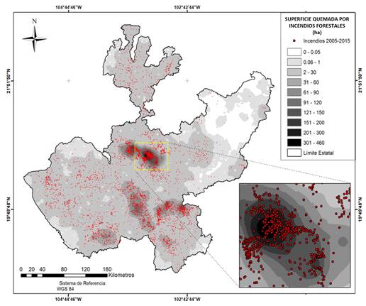
The present research uses information from the state of Jalisco, located in western central Mexico (Figure 1), with a surface area of 78 588 Km², of which 68 % has a warm subhumid climate along the coast and its central area, while 18 % is subhumid temperate, in the higher parts of the mountain chains, and 14 % is dry and semi-dry, in the north and northeast of the state. The mean annual precipitation is approximately 850 mm, although in the coastal zones it is over 1 000 mm per year. According to ^{Rzedowski’s classification (1986}), Jalisco has 13 types of vegetation, most of which consists of pine oak forests and deciduous tropical forests (^{Ramos et al., 2007}).

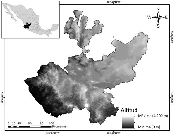
Figure 1 Study area of the sampling unit for determining the spatial variability of the surface area burnt by forest fires in the state of Jalisco, Mexico. 

In Jalisco, the average annual burnt surface ranges between 15 000 and 20 761.58 hectares (^{Conafor, 2015}; ^{Semadet, 2016}). The temperate forest is the most affected, with an annual average of nearly 12 008 hectares; it is followed by the lowland forest and undetermined vegetation, with an average of 1 903.9 hectares; grasslands, with 729.57 hectares; tropical forests, with 463.32 hectares; shrubs, with 190.55 hectares, and montane cloud forests, with 24.27 hectares (^{Conafor, 2016}).

Surface area of reference sites

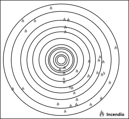
The most convenient minimum sampling surface area for capturing the variability of the average burnt surface was defined in the actual project. For this purpose, a series of circular polygons of twelve different surfaces known as reference sites (RSs) ‒‒1, 2, 4, 8, 10, 15, 30, 50, 70, 100, 150 and 200 Km²‒‒ were analyzed. It was decided that the polygons should be circular because this shape has been used in various forest samplings. Furthermore, circular polygons require only one control point, which facilitates the distribution of the sites (^{McRoberts et al., 1992}). Any geometric figure can be used, as what matters is the size of the site, not its shape.

In order to capture the variability of the average burnt surface, which may occur due to the density of sampling points, four sampling intensities were established: 100, 300, 500 and 1 000. Their location was selected at random, and therefore any point had the same probability of being selected; furthermore, this probability is independent of other points.

Although the spatial independence of the data is outside the scope of this study, it must be analyzed, as through it we seek a low heterogeneity of the variable burnt surface that will ensure the non-existence of spatial autocorrelation. Otherwise, more complex statistic methods integrating the modeling of the spatial structure of the data would have to be applied (^{Zas et al., 2008}). The twelve circular polygons were subsequently located in each reference site (RS).

The next step was to determine how many forest fires have taken place in each RS (Figure 2). For this purpose, statistic information on the forest fires of the 2005-2015 period (^{Conafor, 2015}) was utilized to determine the average burnt surface corresponding to each RS.

Figure 2 Theoretical location of forest fires in reference to the variation of analyzed surfaces for determining the spatial variability of the surface burnt by forest fires in the state of Jalisco. 

Thematic cartography

Once the most adequate RS size was obtained, the corresponding thematic map was generated, illustrating the spatial variation between the surface burnt by forest fires across the state of Jalisco. The interpolation technique known as “weighted inverse distance” --in which the value of an unsampled point is the mean weighted inverse distance between the values of the sampled points-- was used for this purpose (^{Burrough and McDonnell, 1998}). Its interpolation based on the weighted inverse distance is represented by means of the following linear function (^{Flores, 200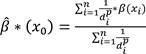1}):

(1)

Where:

* (x ₀ ) = Estimated value at an unsampled site

x ₀ = Location referred to a coordinate system

* (x _i ) = Observed value at a sampled site

x _i, d _i = Distances between each of the sample sites and the unsampled point

p = Exponent of the distance (weighting)

n = Number of sampled sites. In this work, a weighting value (p) of 2 was used, as it best represented the spatial variation of the average burnt surface.

Results

General statistics

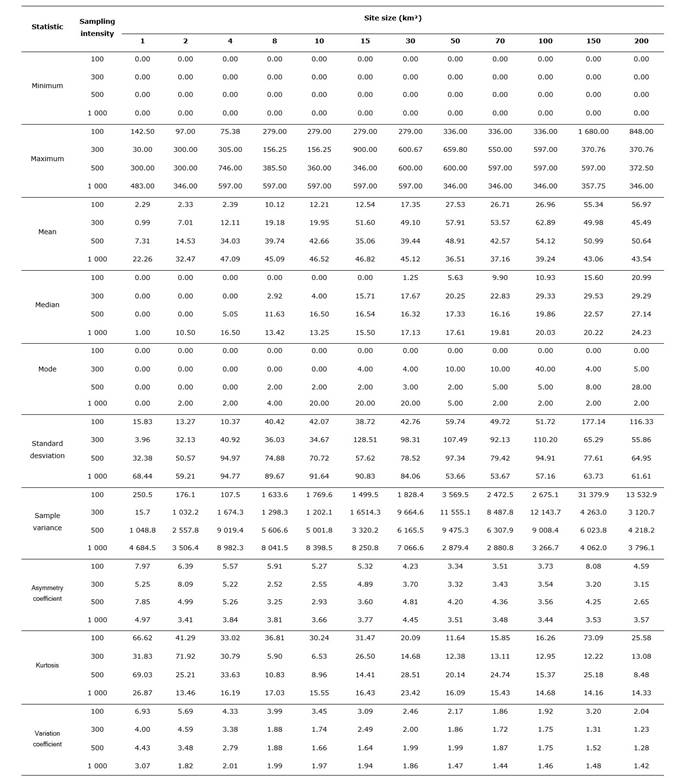
Based on the four sampling intensities (100, 300, 500 and 1 000 sites), the statistics corresponding to the various site sizes were assessed (Table 1). The minimum value, regardless of the size of the site, was observed to be zero burnt hectares, while the maximum burnt surface ranged between 104.9 has (in 1 km²) and 866.66 ha (in 200 km²). In terms of the means and the modes, it was inferred that at most sites there were no burnt surfaces.

Table 1 Statistics of the mean burnt surface by reference site (RS) size in relation to the sampling intensities. 

Sampling unit

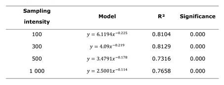
The measure of description was the variation coefficient as a dispersion measure, as it describes the amount of variability (in relation to the mean) without being based on the sample size. Thus, unlike the standard deviation, it was possible to compare the dispersion of the utilized sampling intensities, regardless of the difference between their means. The variability of the average burnt surface decreased in direct proportion to the RS size (Figure 3). This tendency was adjusted to the correlation models corresponding to the sampling intensities (Table 2). This occurred in every case, until an asymptote was reached in which the values of the variation coefficient tended to become stable, which occurs within an interval approximately between 70 and 100 km². Thus, the RS size finally considered as the breaking point of the variability, was 100 km² (radius = 5.650 m), defined as the sampling unit (SU) for the estimation of the spatial variation of the average surface burnt by forest fires.

Table 2 Statistic values to which the tendency of the variation coefficient is adjusted in relation to the site size, for different sampling intensities.  

The Kruskal-Wallis test, a non-parametric equivalent of ANOVA, was utilized to determine the existence of significant differences between the twelve RS sizes for each sampling intensity. Unlike ANOVA, instead of means, the intervals of the RSs are analyzed. First, the data for all RS sizes were combined; subsequently, they were ordered by size, from smaller to larger. The average interval for the data for each RS size was then calculated. The decision criterion applied to accept or discard the null hypothesis that there is no significant difference is the probability value (P). When this is below 0.05, the null hypothesis is discarded.

The resulting probability values are shown in Table 3; at all the intensities, the value of P is below 0.05, which indicates that there is a statistically significant difference between the various RS sizes.

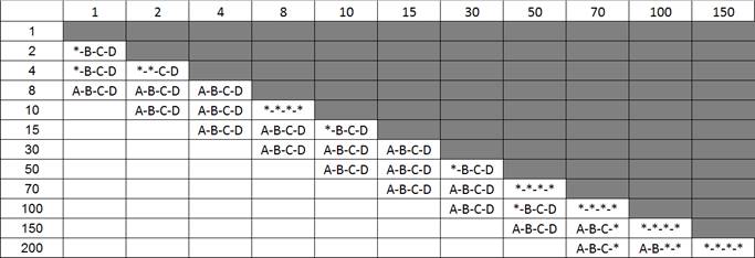
The comparative analysis of paired samples using the Mann-Whitney test determined that there are no differences in the burnt surfaces between RS sizes above and below 100 km² (Table 4), which supports their selection as the breaking point for the asymptotic behavior of the variability (variation coefficient).

Coeficiente de variación = Variation coefficient; Tamaño de sitio = Size site. The vertical line marks the beginning of the asymptotic behavior of the variation coefficient (breaking point [100 km²]).

Figure 3 Tendency of the variation coefficient in relation to site size for different sampling intensities: (A) 100, (B) 300, (C) 500, (D) 1 000. 

Table 3 Results of the Kruskal-Wallis test. 

RS	MR-100	MR-300	MR-500	MR-1000
1	373.92	1 155.5	2023.58	4 325.38
2	380.83	1 244.12	2 108.3	4 556.05
4	408.88	1 304.37	2287.86	4910.26
8	478 215.00	1 457.30	2 461. 56	5 279.23
10	505 035.00	1 496.85	2553.21	5 433.18
15	551 005.00	1 661.44	2 801.95	5 762.49
30	634 455.00	1 860.19	3186.03	6457.73
50	697 695.00	2 048.03	3 435.15	6 844.41
70	739915.00	2189.47	3605.55	7 012.20
100	745 075.00	2 296.35	3 776.34	7 130.64
150	821 955.00	2 415.04	3 862.75	7204.18
200	869.02	2 477.35	3 903.74	7 090.27
H	341.91	903.539	1 235.66	1 528.94
P	0.000	0.000	0.000	0.000

MR = Interval mean (the number indicates the simple size); H= Kruskal-Wallis statistic; P= Probability value.

Table 4 Results of the comparative analysis of paired samples, using the Mann-Whitney test, for the different site (RS) sizes.  

The letters indicate difference in relation to the sampling intensities (P< 0.5): A = 100, B = 300, C = 500, D = 1 000, ^* = without differences between the pairs.

Spatial distribution of the burnt surface

Figure 4 represents the results of this process, which shows a larger burnt surface area (in 100 km²) in the areas where the density of forest fires is higher. Conversely, there were regions with a low or null burnt surface. At the same time, we should note that the density of the number of fires and the spatial variation of the burnt surface area was observed. The highest concentration of fires occurred in central Jalisco, where the highest concentrations of population are located.

Superficie quemada por incendios forestales = Surface burnt by forest fires; Sistemas de referencia = Reference systems

Figure 4 Spatial distribution of the average surface (has) burnt by forest fires, with in an area of 100 km² in Jalisco. 

Discussion

Although several researches define the hazard of fire forests (^{Muñoz et al., 2005}; ^{Yebra et al., 2005}; ^{Rodríguez et al., 2011}), the information (basically in thematic cartography) is generated using various procedures. Notably, the absence of definition of common strategies limits the compatibility and comparability of the results. In order to avoid this, a statistically robust process must be established to determine the burnt surface. For this purposes, it should begin by defining a sampling unit; the present work does so successfully.

Although there are no records of similar researches, it is important to point out that some of the studies specify certain sampling units (^{Carrillo et al., 2012}). Nevertheless, these are not defined statistically but by circumstantial situations. For example, in the work by ^{Carrillo et al., (2012}) addressing the fire hazard criterion, a logistic regression analysis is carried out to establish the most important variables through the random sampling of 10 km² units. However, this unit size is determined only by the spatial resolution of the source information utilized and therefore cannot be used as a comparative sampling unit.

Although there are several studies in which a sampling unit is determined for purposes of forest inventories (^{O'Regan and Arvanitis, 1966}; ^{Zeide, 1980}; ^{McRoberts et al., 1992}; ^{Aguirre et al., 1997}), there are no bases to use this unit in a sampling design to estimate the spatial variability of the surface burnt by forest fires so as to ensure a better location for and sizing of fire management activities. For, taking into account that the task of fighting forest fires is very costly and dangerous, such a unit is very helpful for the management and allocation of resources (^{Díaz et al., 1998}; ^{Rojo et al., 2001}).

A sampling unit allowing the estimation of the spatial variation of the burnt surface in a standardized manner was set. This makes it possible to carry out comparisons between several regions in order to determine priority attention areas. Likewise, the methodology may be used for other types of comparative analyses, e.g. of the temporary variations in the frequency and location of forest fires (^{Rodríguez, 2012}).

The size of the site is defined based on the tendency to the decrease in the variation of the variability (coefficient of variation) of the average burnt surface as the size of RSs increases until it reaches an asymptotic behavior (^{Gallegos et al., 2006}), which occurs in a similar way in the various tested sampling intensities. Thus, an area of 100 km² (radius = 5.650 m) was established as sampling unit (SU) for the estimation of the surface burnt by forest fires. Yet, according to the results, what was determined was not a specific breaking point but an interval (between 70 and 100 km²). In order to standardize a methodological process and ensure that the SU is above the lower limit, an area of 100 km² was selected.

In the process of defining the sampling unit, official statistics for a 10-year period are used (^{Conafor, 2013}). Thus, the georeferentiation of forest fires makes it possible to locate those areas with the highest incidence. These evidences show that, every year, forest fires do not occur in a totally random manner but follow a self-organized critical behavior (^{Torres et al., 2007}; ^{Ávila et al., 2010}; ^{Pérez et al., 2013}). However, a more formal analysis is required to determine an occurrence pattern (^{Ávila et al., 2010}). It may be nevertheless assumed that the average burnt surface does not vary greatly from one year to another. Still, predominant factors such as the variation in the climate conditions and the accumulation of forest fuels must be taken into account. The information on the burnt surface defined using the heat points’ technology can also be incorporated, though with certain reservations, as there is not always a direct relationship between these points and the burnt surfaces (^{Tansey et al., 2008}).

Since the highest frequency of the estimated average burnt surfaces corresponded to low values (<30 ha), and a lower frequency, to 400 ha, the distribution is not normal for all the tested sampling intensities. Notably, a comparative analysis of paired samples established the existence of a significant difference between site sizes within the interval which determines the beginning of the asymptotic behavior of the variability (variation coefficient). Thus, we corroborate that the variability is better captured with the 100 km² site size than with 70 km². This defines a breaking point that is closer to the asymptotic behavior of the variability.

As for the spatial variation of the burnt surface, in locations with a higher density of forest fires, the defined SU was observed to capture a larger number of fires affecting the average burnt surface. The resulting cartography indicates that the largest surfaces are located mainly in central Jalisco. Two important regions to the south and southwest of that state have also been identified. In all of these areas there are large concentrations of population and an important surface is devoted to agricultural and livestock breeding activities; this is relevant, if we consider that most forest fires are caused by anthropic actions. This, in turn, determines geographic patterns of occurrence of fires, based on which priority areas can be delimited in relation to the surface burnt by forest fires (^{Flores et al., 2016a}).

The information thus generated can be utilized both to reinforce and to validate the current determinations of priority hazard areas, which are used for medium- and long-term planning purposes, based on the integral analysis of various parameters, including the temperature, exposure, slope, behavior of the fire, effect of the fire, etc. (^{Flores et al., 2016b}).

Nevertheless, it should be noted that the notion of forest fire hazard must not be mistaken for that of hazard index, which is used for short-term (daily) estimations for operational purposes.

Certain authors suggest defining priority forest fire areas in terms of the spatial variation of their density, using specific processes such as the kernel density function (^{de la Riva et al., 2004}; ^{Kuter et al., 2011}), which is the basis for the estimation of the probability of a high or low density.

Conclusions

The reduction of the variability (variation coefficient) of the average burnt surface observed when the RS size is increased until it displays an asymptotic behavior suggests the acceptance of the initially posed hypothesis. Hence, the sampling unit for the estimation of the variability of the surface burnt by forest fires is 100 km².

The determination of a common sampling unit in order to estimate the spatial variability of the surface burnt by forest fires prevents the lack of correspondence between estimations for different areas.

The results for several areas can be not only compatible but also comparable. I.e., based on the sampling unit (SU), the average burnt surface of a specific area to be sampled can be located, and comparisons can be carried out between several areas. Likewise, the SU makes it possible to share information between different areas, allowing the integration of information in order to determine fire control and prevention strategies in the state of Jalisco or at a regional level.

It is possible to use the determined sampling unit to support the determination of standardized strategies for the validation of forest fire hazard areas, which may be defined using other parameters, such as the temperature, the exposure, the slope, the behavior of the fire, the effect of the fire, etc.

The non-parametric analysis of the data evidences the existence of statistically significant differences between the various site sizes, allowing the determination of the breaking point for the beginning of the asymptotic behavior of the variability, as well as to the establishment of an adequate site size.

As for the spatial variation of the burnt surface, we conclude that the interpolation technique, based on the weighted inverse distance, defines an adequate distribution, as there are spatial coincidences between the highest values for the burnt surface and those areas where the largest concentrations of fire occur.

Although the sample unit was defined using an example at a state level (in Jalisco, Mexico), it can be used in areas with similar conditions. Otherwise, specific sampling units will have to be generated, at a regional, state or municipal level, using the methodology described in this paper. It is suggested to work with statistical data on forest fires for a minimum period of five years.