


Serviços Personalizados
Journal
Artigo
 texto em
  Espanhol (pdf)
 Artigo em XML
 Referências do artigo
 Enviar este artigo por email
Indicadores
-
 Citado por SciELO
 -
 Acessos
Links relacionados
-
 Similares em
SciELO
Similares em
SciELO
Compartilhar

 Permalink
Revista mexicana de ciencias forestales
versão impressa ISSN 2007-1132
Rev. mex. de cienc. forestales vol.8 no.40 México Mar./Abr. 2017
Articles
Cubing system for individual Quercus spp. trees in forests under management in Puebla, Mexico
1 Campo Experimental San Martinito. CIR - Golfo Centro. INIFAP. México. Correo-e: tamarit.juan@inifap.gob.mx
2 Cenid Comef. INIFAP. México.
3 Campo Experimental Valle del Guadiana. CIR - Norte Centro. INIFAP. México.
Taper data of 124 specimens of the Quercus genus were processed. The sample was obtained using the destructive method (felling, limbing and sectioning) in forests under management in the state of Puebla, Mexico. 1 709 pairs of diameter-height data were collected. Each section of the tree was cubed using Smalian’s formula, and the tip by the cone volume formula. The total volume per individual was calculated by adding all its cubed sections. The quality of the statistical adjustment of six segmented taper models was assessed, and the model of Fang et al. (2000) was selected because it best describes the stem profile. The latter was simultaneously adjusted with its expression of commercial volume, using the mixed model technique, and the heteroskedasticity was corrected in the resulting model by weighting the error variance with the exponential function and with a weighting factor in the commercial height exclusively for the taper; the autocorrelation was corrected by modeling the error term; for this purpose, a first-order continuous autoregressive structure (AR(1)) was utilized. The cubing system for individual trees (CSIT) was formed by equations that model the stem profile and estimate the total and commercial volume, as well as the commercial height at a minimum diameter at the tip of the stem, and vice versa. The CSIT makes it possible to carry out volumetric estimations of oak trees per surface area unit.
Key words: Oak forest; product distribution; taper model; stem profile; individual cubing system; commercial volume
Se procesaron datos de ahusamiento de 124 ejemplares del género Quercus. La muestra se obtuvo mediante método destructivo (derribo, desrame y seccionado) en bosques bajo manejo del estado de Puebla, México. Se colectaron 1 709 pares de datos diámetro-altura. Cada sección del árbol se cubicó con la fórmula de Smalian y la punta con la del cono; el volumen total por individuo se obtuvo sumando todas sus secciones cubicadas. Se evaluó la calidad de ajuste estadístico de seis modelos de ahusamiento de tipo segmentado y se eligió el de Fang et al. (2000), que describe mejor el perfil fustal. Este se ajustó, en forma simultánea, con su expresión de volumen comercial, mediante la técnica de modelos mixtos, y en el resultante se corrigió la heterocedasticidad ponderando la varianza de los errores con la función exponencial y un factor de ponderación en la altura comercial, solo para el ahusamiento; la autocorrelación se corrigió modelando el término de error, para ello se usó una estructura continua autorregresiva de primer orden (AR(1)). El sistema de cubicación, a nivel de árbol (SCAI), quedó conformado por ecuaciones que modelan el perfil fustal, estiman el volumen comercial y total, así como la altura comercial a un diámetro mínimo en la punta del fuste y viceversa. El SCAI permite calcular el volumen por tipo de producto según el uso industrial requerido, lo que posibilita realizar estimaciones volumétricas de encino por unidad de superficie.
Palabras claves: Bosque de encino; distribución de productos; modelo de ahusamiento; perfil fustal; sistema de cubicación individual; volumen comercial
Introduction
Mexico has a great diversity of forest species with timber significance, among which those of the Quercus (oak) genus stand out for their abundance, distribution and commercial exploitation. In the year 2013, an oak timber production of 51 461 m3 rw was registered across the country, an amount that represented 8.7 % of the total national timber production, Quercus being the second most important genus, after Pinus (Semarnat, 2014). Although the precise number of Quercus species in Mexico is unknown, Valencia (2004) cites 33 taxa in the state of Puebla, out of 161 identified nationally.
The exploitation of oak timber is a significant source --in terms of both volume and income-- for the silviculturists not only in the state of Puebla but across Mexico. However, in developing forest management programs, models that are over 35 years old are used to estimate the stem volume for Quercus spp. trees. Therefore, studies must be carried out in the state to generate models that may allow accurate estimations of the timber volume, based on rigorous statistic procedures which will prove fair when used as a support for purchase and sale operations.
Today, there is a worldwide consensus on the need to apply, in all the forest systems across the planet, what has been defined as a sustainable forest management, based on an environmentally responsible, socially beneficial and economically viable philosophy (Diéguez-Aranda et al., 2009). A factor that contributes to achieve this goal is the obtainment of volume functions for individual trees as a reliable quantification alternative. Through a wider, better use of statistical techniques, particularly of regression procedures and mathematic modeling, such equations allow considerable cost reductions in the pursuit to optimize the distribution of forest timber products previously to their industrialization, without detriment to the accuracy of the estimations (Pompa-García and Solís-Moreno, 2008).
Total and commercial volume models have recently been developed in Mexico. However, these have been mostly for Pinus species (Corral- Rivas et al., 2007; Hernández et al., 2013; Quiñonez-Barraza et al., 2014), and therefore, volume models for Mexican Quercus species are scarce. The Secretaría de Agricultura y Recursos Hidráulicos (Department of Agriculture and Hydraulic Resources) (SARH, 1978) registers a volume model for oaks in the state of Puebla which is used to estimate the volume in forest inventories. For the state of Chihuahua, Pompa-García and Solís-Moreno (2008) and Pompa-García et al. (2009) developed taper models which, when mathematically integrated, result in an equation for the estimation of the total and commercial value. In the face of this scenario, models and cubing systems must be developed for Quercus under the technical management conditions that are prevalent in the state of Puebla.
For the above reasons, the objective of this work was to develop, based on a segmented taper model, a cubing system for individual trees (CSIT) for oak trees growing in forests under management in that state. The system is a practical, operative technical tool to support decision makers in charge of the management and technical exploitation of this important forest timber resource.
Materials and Methods
The utilized taper and volume data were collected in the Forest Management Units (Unidades de Manejo Forestal, Umafor) 2108, “Chignahuapan-Zacatlán”, and 2101, “Izta-Popo”. The total size of the processed sample consisted of 124 Quercus laurina and Q. rugosa trees of various diameter and height categories, selected in different pruning fronts in forests under management distributed in the study area.
The data were collected using the destructive method. Each selected tree was felled, sectioned and limbed. The measurements of the diameter with bark were recorded in centimeters, and the corresponding heights (HM), in meters, from the base up (level with the ground), at stump height (SH), at 30 cm, and at 60 cm above the stump, and at 1.3 m, with a 5 m StanlerTM flexometer.
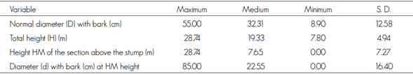
The tree was sectioned at every 2.5 m from the normal diameter up to the total height (H). 1 709 pairs of diameter-height observations distributed along the stems were considered. The normal diameter (D), stump height and total height (H) were obtained separately, and so were the georeferentiation, slope, exposure and altitude of the site from which each tree was collected with a Garmin eTrex type GPS and a Suunto PM-5 Tandem type inclinometer. Table 1 summarizes the basic descriptive statistics of the main variables of the collected sample.
The sections were cubed using Smalian’s formula, and the last section, corresponding to the tip of the tree, was cubed using the cone volume formula. The total stem volume was estimated based on the summation per tree, determined by each of the cubed sections of each tree.


Where:
VS |
= Volume of the section (log) |
S0 and S1 |
= Surface areas (Areas) of the cross-sections of the ends of the section |
L |
= Length of the section |
Vp |
= Volume of the section corresponding to the tip of the tree |
Sb |
= Surface area from the base of the section to the tip of the tree |
h0 |
= Length of the tree tip section |
The taper database was audited before the information was processed. For every tree, charting was used to verify the occurrence of logical behaviors of the variables involving the stem profile and the aggregated volume in relation to the height (Figure 1a and Figure 1b).
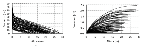
Figure 1 Logical graphic behavior of the stem profile (a) and of the aggregated volume in relation to the height above the stem base (b).
Furthermore, as part of the audit, a chart of the relative diameters (d/Dn) versus relative heights (h/H) (Figure 2) verified the correct logical behavior of the information, for, according to Pompa-García and Solís-Moreno (2008), the range of the data reflects the magnitude of the shape of the trees of which the utilized sample consisted.
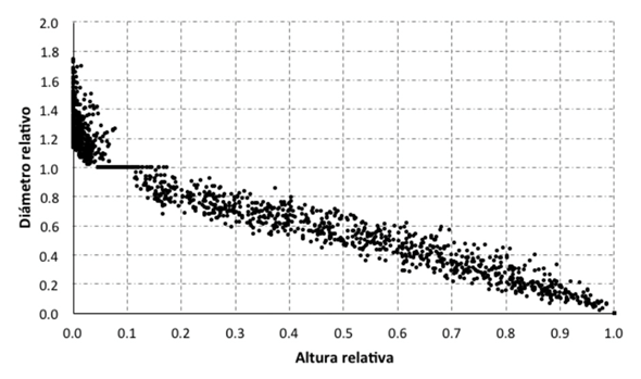
Figure 2 Dispersion of the relative diameters versus the relative heights of the tree sample collected and processed in the adjustment of taper models.
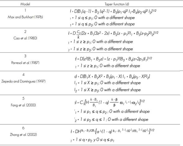
Six segmented taper models (d) (Table 2) were assessed in order to model the stem profile of the Quercus spp. trees, which are characterized by their compatibility with their respective commercial volume function. These models assume that the tree stem is made up of dendrometric body change points (neiloid, paraboloid and cone).
Theoretically, models 1, 2, 4 and 5 assume the existence of two inflection points in the stem, and therefore they suppose that the stem is made up of three geometric forms (segments): the base, as a neiloid; the central part, as a paraboloid, and the tip, as a cone. These models describe the three dendrometric shapes through the adjustment of the equations of the segments described above, which are mathematically joined to form a single taper expression. The rest of the models (3 and 6) assume the existence of a single inflection point.
Table 2 Segmented tapering models evaluated to generate the cubing system for individual Quercus spp. trees.
The various components of the referred models are listed below.
I1 , I2 = Indicator variables for the change of stem dendrometric body
a0 -a2 , B1 -B4 , c0 , p1 , p2 =Parameters to be estimated
The fit of the taper models was carried out using the full information maximum likelihood (FIML) method, with the MODEL procedure of the SAS/ETS® statistical software package (SAS, 2008). The quality of fit of the models was determined by comparing four statistics that are frequently used in forest modeling (Corral-Rivas et al ., 2007; Hernández et al ., 2013; Tamarit et al ., 2014): the adjusted determination coefficient (R2 adj), the bias (E), the root of the mean square error (RMSE), and the Akaike information criterion (AIC), which are expressed as:
Where:
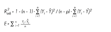

Yi, Ŷi and Ỹi |
= Observed, predicted and mean taper value (d), respectively |
n |
= Total number of observations used to adjust the models |
p |
= Number of parameters of the model to be estimated |
In order to facilitate the eligibility of the best model, besides the four referred statistics, the following were also considered as selection criteria: the sum of squared errors (SSE), the mean square error (MSE) and the likelihood value (logLik).
Based on Sakici et al. (2008), a scoring criterion that consists in organizing the statistics of the models by hierarchy was utilized; for this purpose, consecutive values from 1 to 6 were assigned by order of importance (1 corresponding to the best value of the statistic, and 6, to the most deficient); the total score of each model was estimated according to the summation of the values obtained. The best model was the one with the lowest score.
The best taper model selected was simultaneously adjusted, with its respective commercial value function, in order to profit from the existing compatibility between them, as they share the same parameters. For purposes of comparison in the quality of the fit, the system was first adjusted by non-linear ordinary minimum squares (NLS); then, the mixed effects models technique (MEM) --whose formulation includes the fixed parameters that are common to the entire sample and a specific random parameter for each sampling unit-- was utilized.
The use of MEM improves the quality of the fixed parameters, rendering them more efficient, as they have a lower variance because their errors are low, and, therefore, the estimators are more efficient, accurate and reliable; this allows to make average estimations of the variables of interest with a high level of certainty (De los Santos-Posadas et al., 2006).
Today, MEM has become a common method for analyzing longitudinal data in sites where repeated measurements have been taken of the same experimental unit and the structure of the observations is irregular and imbalanced (Budhathoki, 2006), all of which occurred in the present study.
Based on Hall and Clutter (2004) and on Fang and Bailey (2001), the data were arranged in the form of a bivariate structure that made it possible to include the random effect by incorporating the MEM technique into the adjustment. The compatible taper/volume estimation system was expressed as follows:
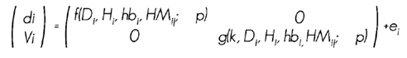
Where:
d1 |
= Observation vector for tapering in the ith tree |
Vi |
= Observation vector for commercial volume in the ith tree |
f(.) |
= Structure of the taper model |
g(.) |
= Commercial volume model |
p |
= Vector for system parameters to be estimated |
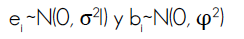
The random effect was defined and included only the parameter B1, which was thus defined in order to control the specific variation at individual tree level, and so, to prevent excess parametrization, overfit of the model and loss of sensitivity of the parameters, given that inferences are based on the latter. It was expressed as follows:
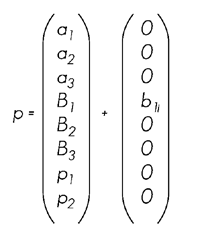
Where:
B1 |
= Only parameter with mixed effect (fixed and random) represented as B1+b1i |
bi |
= Parameter with random effect which, in turn, is defined as: |
Fits were carried out using the NLME package of the R statistical software, version 2.14.0 (R Development Core Team, 2009). In order to compensate potential losses in degrees of freedom and achieve a quicker, more stable convergence in the adjustment of the system with MEM, a restricted maximum likelihood was considered, and the heteroskedasticity and autocorrelation problems were corrected; this allows solid testing of habitual hypotheses regarding the parameters, as well as estimating more realistic confidence intervals (Zimmerman and Núñez-Antón, 2001; Fang and Bailey, 2001).
Heteroskedasticity was corrected through modeling and weighting of the variance of the errors, with the exponential function (e). The weighting factor was based on the HM exclusively for tapering (di), and the commercial volume (Vi) was left constant; the function was structured as:
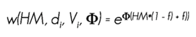
Where:
Φ |
- Parameter to be estimated |
f |
- Indicator variable which takes on the value of 1 for tapering and of 0 for the commercial volumen |
Results and Discussion
Comparison of the fit of taper models
The values of the estimates of the parameters of the six tested tapering models are shown in Table 3. For models 3 and 6, which theoretically assume the existence of a single inflexion point, it was determined that at least one of their parameters was statistically insignificant; this was a sufficient reason to dismiss them without subjecting them to any further analysis.
In models assuming that the stem consists of three geometric shapes (segments), and therefore two inflection points, it was determined that only models 4 and 5 were highly significant in all their parameters; therefore, it is inferred that the stems of the studied oak species exhibit this condition.
Thus, for these models, the first inflection point, where the change from neiloid to paraboloid (p1) occurs, is at 39 % and 4 % of the total height, respectively, while the second (p2), in which the change from paraboloid to cone occurs, is at 89 % and 78 %, respectively.
The results described above are similar to those obtained by Vargas-Larreta (2013) with the model of Fang et al. (2000) for oaks in the state of Chihuahua. The author points out that these changes of geometry occur at 9 and 80 % in relation to the total height of the trees. Models 1 and 2 exhibited insignificant parameters, and therefore they were also dismissed.
Table 3 Estimations of the parameters of the segmented tapering models for describing the diameter profile of oak trees.
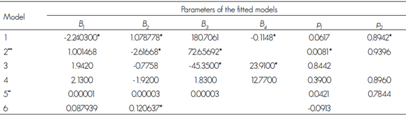
* = Insignificant value;** = Values of the parameters a0, a1, and a2, of 0.00006, 1.96361 and 0.80361 respectively; *** = Value of the parameter c0=0.000197.
Comparatively, model 5 (Fang et al. , 2000) proved to have the best adjustment quality, as its total score was the lowest (Table 4), given its lower values for SSE, MSE, RMSE and AIC, and its higher likelihood (logLik) and R2 adj values. This model accounts for 97.59 % of the total variability of the observed tapering, with the highest accuracy. Furthermore, all the criteria for goodness, except the bias, were the most favorable; therefore, it was selected to describe the stem diameter profile of oak trees.
Table 4 Goodness-of-fit statistics and scores of the taper models for describing the diameter profile of Quercus trees.
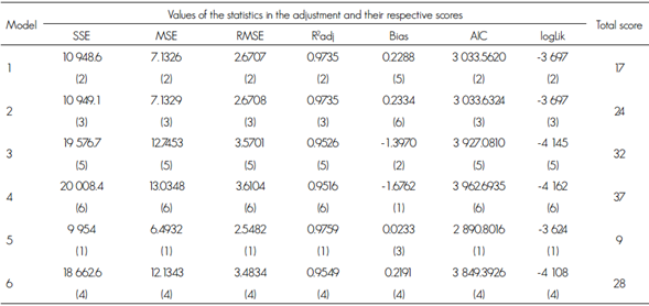
The second best model, even though some of its parameters were insignificant, turned out to be Model 1 (Max and Burkhart, 1976), followed, in order of importance based on the score, by Model 2, proposed by Cao et al. (1980). The models with the lowest adjustment quality were those that assume the existence of a single inflection point.
This is similar to the findings of Corral-Rivas et al. (2007) and Quiñonez-Barraza (2014) for species of the Pinus genus in Durango; it also agrees with the facts documented by Tamarit et al. (2014) for Tectona grandis L. f. established in plantations of southeastern Mexico; for Pinus patula Schiede ex Schltdl. et Cham. in forests under management in Zacualtipan, Hidalgo (Hernández et al., 2013), and for Quercus trees in Chihuahua (Pompa-García et al., 2009). In these cases, the best model was that of Fang et al. (2000), which confirms its high flexibility of adaptation to various species. That the tapering models assuming the presence of three dendrometric bodies in the stem have turned out to be the best may be ascribed, in part, to the fact that the analyzed oak taxa are all from forests under technical management, in which the density and spacing --resulting from the horizontal structure management-- favor the existence of the three dendrometric shapes.
The advantage of the selected model is that it explicitly has a total volume equation, corresponding to the model of Schumacher-Hall (parameters a0, a1, and a2 in the taper function); however, any other with similar structure can be incorporated. Furthermore, it includes an implicit commercial volume equation which, when obtained through analytical integration, is compatible with the taper function; these, then, constitute a system, which can be simultaneously fitted to the model of Fang et al. (2000).
Simultaneous fit of taper/commercial value using NLS and MEM
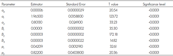
The values of the parameters for the simultaneous adjustment of the taper/commercial value system using NLS for Model 5 turned out to be highly significant, with very low standard errors (Table 5). In this sense, Fang et al. (2000) point out that, when all the parameters of the system are estimated simultaneously, the sum of the total error squares is optimized, which minimizes prediction errors both for the diameter at various heights and of the volume. However, according to Diéguez-Aranda et al. (2009), the choice of the alternative of fitting the system depends on the main use that each of its functions will have, in which case the function of interest must be adjusted independently in order to optimize the estimations of the priority variable.
Table 5 Estimation of the parameters and statistics for the simultaneous fitting of the system constituted by the models of tapering and commercial volume, using NLS.
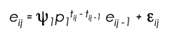
The likelihood ratio test, which compares between the simultaneous adjustments to the system using NLS and MEM, without yet correcting for heteroskedasticity and autocorrelation (MEM-1) turned out to be significant (p < 0.0001), the adjustment being best when MEM is used (Table 6); given the lower values in the Akaike information criterion (AIC) and in the Bayesian information criterion (BIC), as well as the highest value for likelihood (logLik). MEM-3, corrected for heteroskedasticity and autocorrelation, was statistically better than when correction was made only for heteroskedasticity (MEM-2). With this two-fold correction, the MEM residuals are much more homogenous, as proven by the stationarity and insignificance configuration in the first delays (Figure 3); this guarantees that the obtained estimators are not only unbiased but also the most efficient (Myers, 1990; Kozak, 1997).
Table 6 Statistics of the simultaneous adjustment of the system and likelihood test with NLS and with MEM.
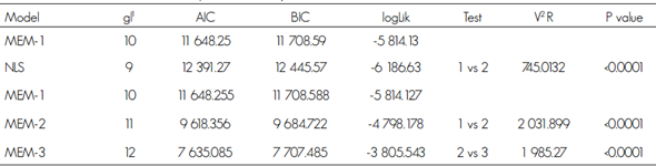
1gl = Degrees of freedom; 2 = Likelihood ratio.
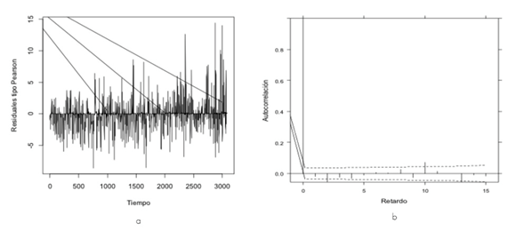
Figure 3 Graphic behavior of the residuals (a) and of the delays (b) after the correction for autocorrelation of the compatible system, using a structure of the AR (1) type.
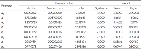
Table 7 shows the simultaneous adjustment of the d-CV compatible system using MEM corrected for heteroskedasticity and autocorrelation (MEM-3) of the highest quality. The intervals for the parameters with fixed effects were narrow, which is indicative of a higher level of demand and a better quality; this evinces that the use of MEM is a favorable refinement in the system adjustment technique that allows making more accurate estimations and inferences of both the tapering and the commercial value.
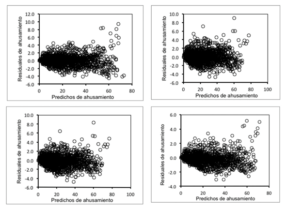
The additional benefit of the adjustment using the MEM approach can be better appreciated when observing the behavior of the residuals versus that of the predicted values, especially in relation to tapering (Figure 4), in which not only does the distribution tend to be random and near zero, but also the scale in the dispersion is lower, comparatively, with the residuals of the adjustment using NLS. In this respect, Fang and Baily (2001) point out that, under the MEM approach, it is possible to improve the characteristics of the parameters by compensating for the effect of variables measured in the same experimental unit. This approach takes into account the contemporary correlation, which helps reduce the standard errors of the model’s parameters considerably and allows unifying the values by component.
Table 7 Fixed estimated parameters and goodness-of-fit of Model 5 corrected for heteroskedasticity and autocorrelation (MEM-C).
According to Diéguez-Aranda et al. (2006) and to Li and Weiskittel (2010), the behavior of the segmented model of Fang et al. (2000) is good for estimating both the total volume and the diameters at various heights in conifer trees with differently sized normal diameter and total height.
Cubing system for Quercus spp. Trees
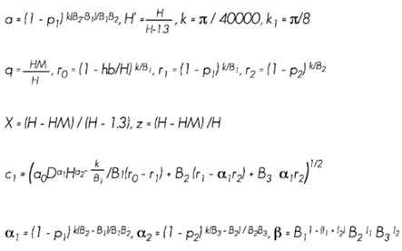
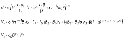
The cubing system for individual trees (CSIT) for Quercus spp. consists of the taper expression d (model 5), of the function estimating the commercial volume (CV) proposed by Fang et al. (2000), as well as of the corresponding expression to estimate the commercial height (HM) at a minimum commercial diameter (d), and the total volume (V) equation. The CSIT is expressed as follows:
The total volume equation corresponding to the model of Schumacher-Hall, defined in terms of the normal diameter and total height, facilitates the construction of a table for the total stem volume. On the other hand, with the combination of the rest of the equations, it is possible to estimate the commercial volume at a minimum diameter at the tip of the stem, as well as the height at which a particular diameter is attained according to the requirements of the industry and the commercial use.
A comparison between the model for estimating the total volume of Quercus spp. in Chihuahua proposed by Pompa-García and Solís-Moreno (2008) --derived by these from a taper model and consistently corresponding to the factor model (V=0.25226855D2H)-- and the one generated in the present study by Schumacher Hall (V=0.0000427D1.7339635H1.2070785), based on a taper model, proves that the former tends to produce underestimations, while the latter produces more consistent total volume estimates that are closer to the observed volumes; this shows the usefulness and benefit of generating this type of models and cubing systems for specific regions where the timber-yielding species of commercial interest grow and thrive.
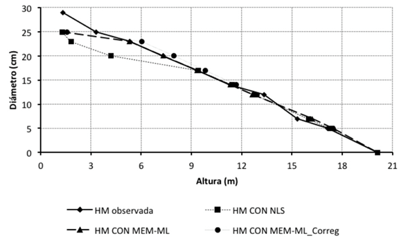
The generated CSIT meets the following condition: if the minimum diameter is zero, then the commercial value is equal to the total value, as the commercial height equals the total height. Thus, for a Quercus tree with a D of 29 cm and a H of 20 m, the system cubes a total stem volume of 0.54 m3, which is close to the observed volume, of 0.539 m3. When a minimum commercial stem diameter of 20 cm is considered, a HM of 7.91 m is estimated; the CV corresponding to these specifications, and from the stump up, is 0.41 m3.
Figure 5 shows the above data in a graphic form, as well as the functioning of the system for the estimation of the commercial height with the various utilized adjustment techniques. Based on the values of the CSIT parameters, it is possible to generate volume tables by product type and, thus, to estimate both the commercial volume and its monetary value in terms of the market price.
Conclusions
For the six assessed taper functions, the model of Fang et al. (2000) has a superior performance, as it best describes the data used in the adjustment; therefore, it is recommended as the best model to describe the stem diameter profile and for cubing individual Quercus spp. trees in forests under management in the state of Puebla. This model, along with its respective commercial and total volume functions, constitutes a cubing system for individual trees (CSIT) of this genus.
The adjustment strategy with the mixed effect model technique is superior to that of ordinary minimum squares, as it provides more accurate and consistent estimations in the calculation of the commercial and total volume, as well as of the minimum commercial diameters at various heights, and vice versa.
The cubing system that was made is a basic tool to apply it in the forest inventories in the Umafores and the study region; they are useful for economic stand assessments, and as a support for planning the final use of the harvested stems, according to industrial requirements.
Referencias
Budhathoki, C. B. 2006. Mixed-effects modeling of shortleaf pine (Pinus echinata Mill.) growth data. Thesis for doctor of philosophy. Oklahoma State University, Stillwater, OK, USA. 168 p. [ Links ]
Cao Q., V., H. E. Burkhart and T. A. Max. 1980. Evaluation of two methods for cubic-volume prediction of loblolly pine to any merchantable limit. Forest Science 26(1): 71-80. [ Links ]
Corral-Rivas, J. J., U. Diéguez-Aranda, S. Corral Rivas and F. Castedo-Dorado. 2007. A merchantable volume system for major pine species in El Salto, Durango (Mexico). Forest Ecology Management 238: 18-129. [ Links ]
De los Santos-Posadas, H., M. Montero-Mata y M. Kanninen. 2006. Curvas dinámicas de crecimiento en altura dominante para Terminalia amazonia (Gmel.) Excell en Costa Rica. Agrociencia 40: 521-532. [ Links ]
Diéguez-Aranda, U., F. Castedo-Dorado, J. G. Álvarez G. and A. Rojo. 2006. Compatible taper function for Scots pine plantations in northwestern Spain. Canadian Journal Forest Research 36(5): 190-1205. [ Links ]
Diéguez-Aranda, U ., A. Rojo A., F. Castedo-Dorado, J. G. Álvarez G., M. Barrio-Anta, F. Crecente-Campo, J. M. González G., C. Pérez-Cruzado, R. Rodríguez S., C. A. López-Sánchez, M. Á. Balboa- Murias, J. J. Gorgoso V. y F. Sánchez R. 2009. Herramientas selvícolas para la gestión forestal sostenible en Galicia. Universidad de Santiago de Compostela. Galicia, España. 259 p. [ Links ]
Fang, Z., B. E. Borders and R. L. Bailey. 2000. Compatible volume-taper models for loblolly and slash pine based on a system with segmented-stem form factors. Forest Science 46(1):1-12. [ Links ]
Fang, Z. and R. L. Bailey. 2001. Nonlinear mixed effects modeling for slash pine dominant height growth following intensive sivicultural treatments. Forest Science 47(3): 287-300. [ Links ]
Hall, D. B. and J. L. Clutter. 2004. Multivariate multilevel nonlinear mixed effects models for timber yield predictions. Biometrics 60(1):16-24. [ Links ]
Hernández P., D., H. M. De los Santos P., G. Ángeles P., J. R. Valdez L. y V. H. Volke H. 2013. Funciones de ahusamiento y volumen comercial para Pinus patula Schltdl. et Cham. en Zacualtipán, Hidalgo. Revista Mexicana de Ciencias Forestales 4(16): 35-45. [ Links ]
Kozak, A. 1997. Effects of multicollineariy and autocorrelation on the variables exponent taper functions. Canadian Journal Forest Research 27: 619-629 [ Links ]
Li, R. and A. R. Weiskittel. 2010. Comparison of model forms for estimating for stem taper and volume in the primary conifer species of the North American Acadian Region. Annals of Forest Science 67(3): 302. [ Links ]
Max, T. A. and H. E. Burkhart. 1976. Segmented polynomial regression applied to taper equations. Forest Science 22(3): 283-289. [ Links ]
Myers, R. H. 1990. Classical and modern regression with applications. 2nd ed. Duxbury Press. Belmont, CA, USA. 488 p. [ Links ]
Parresol, B., J. Hotvedt and Q. Cao. 1987. A volume and taper prediction system for bald cypress. Canadian Journal Forest Research 17(3):250-259 [ Links ]
Pompa-García, M. y R. Solís-Moreno. 2008. Ecuación de volumen para el género Quercus en la región noroeste de Chihuahua, México. Quebracho 16: 84-93 [ Links ]
Pompa-García, M ., J. J. Corral-Rivas, J. C. Hernández-Díaz and J. G. Álvarez- González. 2009. A system for calculating the merchantable volume of oak trees in the northwest of the state of Chihuahua, Mexico. Journal of Forestry Research 20(4): 293-300. [ Links ]
Quiñonez-Barraza, G., H. M. De los Santos-Posadas, J. G. Álvarez-González y A. Velázquez-Martínez. 2014. Sistema compatible de ahusamiento y volumen comercial para las principales especies de Pinus en Durango, México. Agrociencia 48: 553-567. [ Links ]
R Development Core Team. 2009. R: a language and environment for statistical computing. R Foundation for Statistical Computing. Vienna, Austria. ISBN 3-900051-07-0. URL: URL: http://www.R-project.org (24 de abril de 2015). [ Links ]
Sakici, O. E., N. Misira, H. Yavuza and M. Misira. 2008. Stem taper functions for Abies nordmanniana subsp. bornmulleriana in Turkey. Scandinavian Journal of Forest Research 23(6): 522-533. [ Links ]
Secretaría de Agricultura y Recursos Hidráulicos (SARH). 1978. Inventario forestal del estado de Puebla. Subsecretaría Forestal y de la Fauna. Dirección General del Inventario Forestal. Núm. 44. México, D. F., México. 50 p. [ Links ]
Statistical Analysis System (SAS). 2008. SAS/STAT® 9.2 User’s Guide. SAS Institute Inc. Raleigh, NC, USA. n/p. [ Links ]
Secretaría del Medio Ambiente y Recursos Naturales (Semarnat). 2014. Anuario Estadístico de la Producción Forestal 2013. México, D. F., México. 230 p. [ Links ]
Tamarit U., J. C., H. M. De los Santos P.,A. Aldrete, J. R. Valdéz L., H. Ramírez M. y V. Guerra de la C. 2014. Sistema de cubicación para árboles individuales de Tectona grandis L. f. mediante funciones compatibles de ahusamiento-volumen. Revista Mexicana de Ciencias Forestales 5(21): 58-74. [ Links ]
Valencia A., S. 2004. Diversidad del género Quercus (Fagaceae) en México. Boletín de la Sociedad Botánica de México 75: 33-53 [ Links ]
Vargas-Larreta B. y J. J. Corral-Rivas. 2013. Validación y calibración del sistema biométrico utilizado en la elaboración de programas de manejo forestal maderable en la UMAFOR 0808 “Guadalupe y Calvo”, Chihuahua. Comisión Nacional Forestal. San Juan de Ocotán, Jal., México. Informe técnico. 50 p [ Links ]
Zepeda B., E. M. y A. Domínguez P. 1997. Ecuaciones de ahusamiento para tres especies de pino, del ejido El Largo, Chihuahua. In: Memoria de resúmenes de ponencias. III Congreso Mexicano sobre Recursos Forestales. Linares, NL., México. 43 p. [ Links ]
Zhang, Y., B. E. Borders and R. L. Bailey. 2002. Derivation, fitting, and implication of a compatible stem taper-volume-weight system for intensively managed, fast growing loblolly pine. Forest Science 48(3):595-607. [ Links ]
Zimmerman, D. L. and V. Núñez-Antón. 2001. Parametric modelling of growth curve data: an overview (with discussion). Test 10(1): 1-73 [ Links ]
Received: July 22, 2016; Accepted: March 12, 2017
 Este es un artículo publicado en acceso abierto bajo una licencia Creative Commons
