


Servicios Personalizados
Revista
Articulo
 texto en
  Inglés (pdf)
 Artículo en XML
 Referencias del artículo
 Enviar artículo por email
Indicadores
-
 Citado por SciELO
 -
 Accesos
Links relacionados
-
 Similares en
SciELO
Similares en
SciELO
Compartir

 Permalink
Revista mexicana de ciencias forestales
versión impresa ISSN 2007-1132
Rev. mex. de cienc. forestales vol.8 no.39 México ene./feb. 2017
Articles
Inventory and mapping of a pine forest under timber management using data obtained with a SPOT 6 sensor
1Posgrado en Ciencias Forestales. Colegio de Postgraduados. Campus Montecillo. México. Correo-e: valdez@colpos.mx.
2Facultad de Ingeniería. Universidad Autónoma de San Luis Potosí. México.
The purpose of the present research was to quantify and map the forest density, basal area (BA), total biomass (Bt), crown cover (CC), volume (Vol) and leaf area index (LAI) variables in a Pinus patula forest under timber management. Initially, the existing correlations between the spectral data derived from the SPOT-6 satellite sensor and field inventory data were identified. The analysis included the use of multiple linear regression models, ratio and regression estimators, and the traditional inventory approach (with field data only), for comparative purpose. The highest correlations for BA, Bt, CC and Vol were obtained using the near infrared strip; the values were 0.74, -0.77, -0.50 and -0.77, respectively, while the LAI had the highest correlation with the green strip, having a value of -0.65. The best adjustments were obtained for the regression models predicting the BA, Bt and Vol variables, a R2 adj of 0.66 for each variable, and mean square root error (MSRE) values of 5.82 m2 ha-1, 32 Mg ha-1 and 62.3 m3 ha-1 respectively. Inventory estimations were undertaken using the ratio and regression estimators’ method, being within the range of the confidence interval of the random sampling. The regression estimator registered the following precision values: 4.8 % (BA), 6.7 % (Bt), 5.8 % (CC), 6.6 % (Vol), 6.9 % (LAI). This type of sampling turned out to be the most conservative of all that were carried out.
Key words: Total biomass; leaf area index; forest inventory; spatial modeling; Pinus patula Schiede ex Schltdl. & Cham.; density variables
El objetivo de la investigación fue cuantificar y mapear las variables de densidad forestal, área basal (Ab), biomasa total (Bt), cobertura de copa (Cob), volumen (Vol) e índice de área foliar (IAF) en un bosque de Pinus patula bajo manejo maderable. Inicialmente, se identificaron las correlaciones existentes entre los datos espectrales derivados del sensor satelital SPOT 6 y datos de campo del inventario. El análisis incluyó el uso de modelos de regresión lineal múltiple, estimadores de razón y regresión y el enfoque tradicional de inventario (solo con datos de campo), con fines comparativos. Las correlaciones más altas para Ab, Bt, Cob y Vol fueron con la banda del infrarrojo cercano; los valores fueron de 0.74, -0.77, -0.50 y -0.77, respectivamente. Mientras que el IAF presentó la mayor correlación en la banda verde con un valor de -0.65. Los mejores ajustes se lograron para los modelos de regresión que predicen las variables Ab, Bt y Vol; R2 adj de 0.66 para cada una de ellas y valores de raíz del error medio cuadrático (REMC) de 5.82 m2 ha-1, 32 Mg ha-1 y 62.3 m3 ha-1 respectivamente. Las estimaciones de inventario se calcularon mediante el método de estimadores de razón y de regresión, y estuvieron dentro de la amplitud del intervalo de confianza del muestreo aleatorio. El estimador de regresión registró valores de precisión: 4.8 % (Ab), 6.7 % (Bt), 5.8 % (Cob), 6.6 % (Vol), 6.9 % (IAF). Este tipo de muestreo resultó el más conservador de todos los realizados.
Palabras clave: Biomasa total; índice de área foliar; inventario forestal; modelación espacial; Pinus patula Schiede ex Schltdl. & Cham.; variables de densidad
Introduction
The evaluation and management of forest resources require these to be quantified by means of forest inventories, which are obtained through in-field samplings that include the assessment of certain variables like forest density, tree height, crown cover, basal area, and timber-yielding volume; at the same time, they involve significant effort and costs (Hawbaker et al., 2010; Tanaka et al., 2014).
Geomatics includes disciplines such as remote perception, geographic information systems (GIS), and global navigation satellite systems (GNSS), which facilitate the collection of worthy and timely data and information about the natural resources, providing an alternative to forest inventories. These technologies make it possible to estimate variables both locally (Ortiz-Reyes et al., 2015) and in large areas at various levels of detail and in less time (Merem and Twumasi, 2008; Muñoz-Ruiz et al., 2014).
Constant progress in computer science makes it possible for remote sensors, mounted on satellite platforms or aircrafts, to capture images at ever shorter time intervals, with better spatial and spectral resolution (Ikonos, QuickBird, SPOT 6 and 7, Pléiades), making timely data and information available for the planning and management of forest resources, particularly in areas with a difficult access (Valdez-Lazalde et al., 2006).
In this regard, the technology associated to geomatics can be used to estimate forest inventories and to transform these visual results (e.g. maps) for purposes of decision making in the management of the resources. The objective of the present study was to map the basal area, total biomass, volume, crown cover and leaf area index of a Pinus patula forest under timber management, using spectral data from the SPOT-6 sensor in Zacualtipán, Hidalgo, Mexico, in order to compare the traditional inventory with the remote sensing-assisted inventory.
Materials and Methods
Study area
The study area is located in Zacualtipán de Ángeles municipality, in the state of Hidalgo, Mexico, between the coordinates 20°36’00” and 20°37’40” N, and 98°34’44” and 98°36’32” W (Figure 1). It covers a surface area of 900 ha (3 x 3 km). Its physiography includes part of the High Sierra of Hidalgo and the Neovolcanic Axis, in the Carso Huasteco subprovince, and is constituted by slopes, plateaus and canyons. The edaphic substratum consists of Orthic acrisol (Ao), Chromic Luvisol (Lc), and Haplic phaeozem (Hh). The existing climate is temperate-humid [C(fm)w”b(e)g], with a marked rainy season between June and October. Precipitation is approximately 2 050 mm (INAFED, 2015).
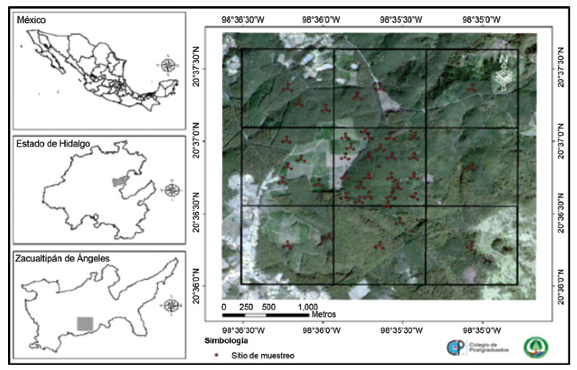
Figure 1 Location of the Pinus patula Schiede ex Schltdl. & Cham. forest in Zacualtipán de Ángeles, Hidalgo.
In the last decades, the area has been managed using the Silvicultural Development Method (MDS), which gave rise to mono-specific, coetaneous Pinus patula stands with various covers and ages ranging from 0 to 31 years. There are also stands without silvicultural intervention (i.e. natural), aged approximately 80 years. Although the intervened stands are technically characterized as mono-specific, they include a minimal proportion of other species in a varied distribution: primarily P. teocote Schiede ex Schltdl. & Cham., Prunus serotina Ehrh., Quercus laurina Bonpl., Q. rugosa Née, Q. excelsa Liebm., Q. crassifolia Bonpl., Q. affinis Scheidw., Cornus disciflora Moc. & Sessé ex DC., Viburnum spp., Cleyera theaoides (SW.) Choisy, Alnus jorullensis Kunth, Arbutus xalapensis Kunth, Symplocus spp., Ternstroemia spp. and Vaccinium leucanthum Schltdl. (Figueroa et al., 2010).
In-field sampling
A systematic sampling system under a cluster design similar to the one proposed by the National Forestry Commission (Comisión Nacional Forestal) (Conafor, 2011) for the National Forest and Soil Inventory (Inventario Nacional Forestal y de Suelos, INFyS) was utilized. Each cluster consists of four 400 m2 sites arranged in the shape of an inverted “Y” (Figure 1). The sample comprised 157 sites belonging to the Atopixco Intensive Carbon Monitoring Site, in the state of Hidalgo. These sites are monitored because they are part of the Mexican Network of Intensive Carbon Monitoring Sites (Ángeles-Pérez et al., 2012).
The inventory was carried out in May, 2013, and measured the following variables in all the trees present: normal diameter (ND at 1.30 m above ground level), total height (Ht) and crown diameter (CD).
Estimation of the forest density variables
The variables measured in field served as a basis to estimate the basal area (BA), total biomass (Bt), crown cover (CC), volume (Vol) and leaf area index (LAI) of individual trees using mathematical models. The estimates at tree level were added up in order to obtain the values per site. The basal area was calculated using the following formula:

The total biomass and volume were determined based on the models adjusted by Cruz (2007) and Soriano-Luna et al. (2015) for the study area (Table 1).
Table 1 Models for estimating the total biomass (Bt) and Volume (Vol) in Zacualtipán de Ángeles, Hidalgo.

Bt in kg; Vol in m3; ND = Normal diameter in cm; Ht = Total height in m
The crown cover (CC) was estimated based on the average crown diameter (CD), which in turn was calculated by measuring the crown diameter in two directions (N-S and E-W), with the equation:

Where:
CC in m2
CD in m
The LAI for P. patula was estimated with the model used by Aguirre-Salado et al. (2011):
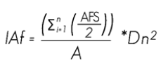
Where:
LAI |
= in m2 m-2 |
LSA |
= Leaf surface area in m2 |
A |
= Sampling site surface area (400 m2) |
i |
= ith tree of the sampling site |
The calculation of the LSA requires knowing the values of the specific leaf area (SLA) and the dry leaf biomass (DLB) of each of the trees within the sampling site (Aguirre-Salado et al., 2011). The models shown in Table 2 were used for this purpose.

Preprocessing of the SPOT-6 image
The SPOT-6 image was captured in January, 2014, because the poor atmospheric conditions made it impossible to capture them on a nearer date to the in-field sampling period. Although there is a time lag between the field data and the spectral data, the analysis is adequate because this lag is short, considering the growth rate of the forest mass; besides, the intention was to estimate the inventory as of the date of the in-field data collection, i.e. May, 2013.
The SPOT-6 image has a spatial resolution of 6 m in multispectral mode, and a Standard Ortho process, which consists in an ortho-rectification using a digital elevation model (DEM), and a 12-bit radiometric correction using the nearest neighbor method (Astrium, 2013).
The spectral data (digital numbers) were converted to irradiance values and, in turn, to reflectance values. The ArcMapTM version 10.2 package was used for this purpose, with the following formulas (Astrium, 2013):


Where:
L b (p) |
= Irradiance at the top of the atmosphere (w sr-1 m-2 µm-1) |
DC(p) |
= Digital number |
GAIN(b) |
= Gain calibration coefficient of each band |
BIAS(b) |
= Multiplicative factor of the band |
Pb(p) |
= Adimensional exoatmospheric reflectance |
π |
= Value of number pi (3.1416) |
E 0 (b) |
= Mean solar exoatmospheric irradiance of each band |
Cos(ϴs) |
= Cosine of the solar zenith angle of the scene (90° - ϴs) |
The values of the parameters were obtained from the metadata of the SPOT-6 image.
Estimation of the spectral variables
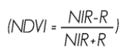
The spectral variables used were the four bands of the SPOT-6 image: blue (B), green (G), red (R) and near infrared (NIR) (Astrium, 2013). In addition, the normalized differences vegetation index was calculated, because it has a high correlation with the vegetation cover (Aguirre-Salado et al., 2011).
These variables were extracted as the average reflectance of each of the sampling sites (400 m2) established in field, using the Zonal Statistics as Table command of the ArcMapTM version 10.2 software.
Statistical analysis
In principle, the field data at site level were transformed by calculating the square root of their original value in order to minimize the variance and obtain a normal distribution. Pearson’s correlation coefficient implemented in the SAS 9.0TM software was subsequently estimated in order to identify the spectral variables correlated with the field variables.
The stepwise regression method was then applied to identify the adequate multiple linear regression models for estimating the basal area, total biomass, crown cover, volume and leaf area index at site level. The structure of the models was as follows:

Where:
Y |
= Variable of interest |
X n |
= Spectral variables with reflectance values |
β n |
= Regression parameters |
ε i |
= Error |
The goodness-of-fit indicators considered for the selection of the best models were the adjusted determination coefficient (R2 adj), the Mean Square Root Error (MSRE) and a rejection probability value (p) below 0.05 for each of the regression parameters.
The traditional inventory of the BA, Bt, CC, Vol and LAI variables was carried out with two types of sampling: simple random and stratified (Scheaffer et al., 1986); of these, the one that yielded the most accurate values was used as a point of comparison for the estimations based on spectral data of the SPOT-6 sensor.
The criterion for the selection of the best traditional inventory vs. the remote sensing inventory was the precision attained in the estimations, while the criterion within the remote-sensing inventories was the Mean Square Root Error (MSRE).
Given the high correlation that usually exists between the field variables and certain spectral variables (Aguirre-Salado et al., 2009; Muñoz-Ruiz et al., 2014), the data registered in the SPOT-6 served as a base to estimate, through interpolation, the values of the variables for the whole study area at pixel level, by means of ratio and regression estimators (Scheaffer et al., 1986; Valdez-Lazalde et al., 2006).
The best adjusted regression models were utilized to generate thematic maps of the variables of interest (BA, Bt, CC, Vol and LAI) with map algebra, using the ArcMapTM version 10.2 software.
Results and Discussion
Relationship between field and spectral variables
The correlation of the field variables and the spectral variables was negative; that is, the higher the value of the field variable, the lower the value of the spectral variable (Table 3). The correlations range between -0.36 and -0.77, and the CC stands out as the only field variable having correlations below or equal to -0.50.
Table 3 Correlation matrix of the field variables vs. spectral variables.

BA = Basal area; Bt = Total biomass; CC = Crown cover; Vol = Volume; LAI = Leaf area index; B = Blue band; G = Green band; R = Red band; NIR = Near infrared band; NDVI = Normalized difference vegetation index. All the correlations were highly significant (0.001).
The spectral variable that had the highest correlation with the field variables was the NIR band (Table 3); its incorporation into the multiple linear regression models was therefore considered. In general, the behavior of the NIR band consisted in showing high reflectance values for those areas with dense, vigorous vegetation. Low values corresponded to the opposite vegetation conditions (i.e. sparse or weak vegetation), as well as to water bodies, which absorb the reflectance, or areas with a high moisture content (Chuvieco, 1995). The highest correlations for BA, Bt, CC and Vol were obtained with the NIR band, the values being -0.74, -0.77, -0.50 and -0.77, respectively, while the highest correlation for LAI occurred in the G band, with a value of -0.65.
These negative tendencies are similar to those cited by Aguirre-Salado et al. (2011) for a P. patula forest under timber management, located in the vicinity of the area covered by the present study. These authors indicate a correlation of -0.92 and -0.93 for CC between the NIR band and the LAI, while the G band has a correlation of -0.40 and -0.39 for LAI and CC, respectively.
The low correlation recorded in the research that is documented is due to two situations at the sampling sites: 1) sites with bare soil were not considered, in order to provide the model with as many observations with zero tendency (Aguirre-Salado et al., 2011); and 2) the high diversity of species that have the sites, since the NIR band captures the structure of the cells and the moisture (Jensen, 2007).
A different case was registered by Muñoz-Ruiz et al. (2014) in the temperate forests of the state of Hidalgo, where the G band had correlations of -0.43 for BA, -0.31 for CC and -0.47 for Vol, while the correlation with the NIR band was very low, with 0.03 for BA, 0.15 for CC and 0.03 for Vol. In the mesophile forests, the G band showed values of -0.46 for BA, 0.08 for CC and -0.44 for Vol, and the NIR band exhibited values of -0.36 for BA, 0.04 for CC and -0.33 for Vol.
Estimations of variables using regression models
Given the high correlation of the NIR band with the field variables, this was considered as an independent variable for purposes of adjusting multiple linear regression models. The best adjustments were attained for the models predicting the BA, Bt and Vol variables with a R2 adj of 0.66 for each variable and a MSRE of 5.82 m2 ha-1, 32 Mg ha-1 and 62.3 m3 ha-1, respectively. The CC had the lowest adjustment, with a R2 adj of 0.27 and a MSRE of 35.03 %. A R2 adj of 0.51 and a MSRE of 2.07 m2 m-2 were obtained for the LAI (Table 4).
Table 4 Multiple linear regression models for the field variables (FV), in Zacualtipán de Ángeles, Hidalgo.

BA = Basal area; Bt = Total biomass; CC = Crown cover; Vol = Volume; LAI = Leaf area index; B = Blue band; R = Red band; NIR = Near infrared band; NDVI = Normalized difference vegetation index; MSRE = Mean Square Root Error; A0, A1, A2, A3, A4 = Parameters of the model. All the parameters were significant (0.05).
Cruz-Leyva et al. (2010) adjusted regression models to predict similar variables in P. patula and P. teocote forests under timber management, in Zacualtipán de Ángeles, Hidalgo, based on data of the SPOT-5 sensor, with good adjustments to produce the BA (R2 adj = 0.96). This is because the cartographic variables of altitude (masl) and mean annual temperature had a good correlation with the spectral variables. Velasco et al. (2010) estimated the LAI in Abies religiosa forests of the Monarch Butterfly Biosphere Reserve in Michoacán using spectral data of the SPOT-4 sensor; its adjustment turned out to be lower (R2 adj = 0.61, with a MSRE = 0.493). Aguirre-Salado et al. (2011) used linear regression models to predict LAI and CC based on SPOT-5 HRG data, in a smaller surface area near the study area, with good adjustments although they only utilized the R band: R2 adj = 0.92 for LAI and R2 adj = 0.93 for CC.
Except for the model utilized for the CC, the rest of the multiple linear regression models, selected using STEPWISE, had an acceptable graphic adjustment. When charting the observed values vs. the predicted values, a rising tendency is observed, i.e. the higher the value of the data observed in field, the higher the value of the data predicted through remote sensing (Figure 2).

Figure 2 Dispersion chart of observed vs. predicted data for the basal area (BA), total biomass (Bt), crown cover (CC), volume (Vol) and leaf area index (LAI).
The MSREs registered by the multiple linear regression models were 5.82 m2 ha-1 for BA, 32 Mg ha-1 for Bt, 35.03 % for CC, 62.30 m3 ha-1 for Vol and 2.07 m2 m-2 for LAI (Table 4); these values are similar to those recorded by Aguirre-Salado et al. (2009) --4.2 m2 ha-1 for BA and 57.71 m3 ha-1 for Vol--, obtained with multiple linear regression models for P. patula in Hidalgo. Velasco et al. (2010) point out an error of 0.493 m2 m-2 in the LAI using multiple regression models for sacred fir forests of the Monarch Butterfly Biosphere Reserve in Michoacán. Aguirre-Salado et al. (2011) indicate errors of 0.50 m2 m-2 for LAI and of 5.71 % for CC, using simple linear regression models for P. patula forests under timber management in Zacualtipán de Ángeles, Hidalgo. The MSRE values obtained by Muñoz-Ruiz et al. (2014) with multiple linear regression models were 6.70 m2 ha-1 for BA, 41.45 m3 ha-1 for Vol and 29.69 % for CC in temperate forests, and 8.5 m2 ha-1 for BA, 29 % for CC and 79.14 m3 ha-1 for Vol in mesophile forests of the state of Hidalgo.
Estimation of the traditional inventory
The simple random sampling system showed more precision (error below 10 %) in the estimations of the dasometric variables, obtaining total inventories of 21 022.65 m2 for BA; 80 430.49 Mg for Bt; an average of 102.28 % for CC; 156 932.22 m3 for Vol; and 3.24 m2 m-2 for LAI (Table 5).
Table 5 Total inventory estimations for the Pinus patula Schiede ex Schltdl. & Cham. forest under timber management in Zacualtipán de Ángeles, Hidalgo, using different analysis strategies.

SRS =Simple random sampling; SS =Stratified sampling; SRatE = Sampling with ratio estimator; SRegE =Sampling with regression estimator; CI+ =Upper confidence interval; CI- =Lower confidence interval.
These results are similar to those obtained by Ortiz-Reyes et al. (2015) for the same study area, but they were calculated based on LiDAR data. These authors estimated 20 787.40 m2 for BA; 104 037.86 Mg for Bt; an average of 131.54 % for CC, and 163 436.48 m3 for Vol in a surface area of 913 ha. For a neighboring area, Aguirre-Salado et al. (2011) registered an average value of 80 % for CC and of 6 m2 m-2 for LAI in mature P. patula forests (aged 20 - 24 years).
The differences in the estimations of CC and LAI described above are partially due to the constantly occurring forestry interventions (total or partial harvesting of different intensities) in the forest that was the subject of this study. Furthermore, it should be mentioned that the estimations of Bt and Vol were carried out using regression models updated as of 2015 for the work area.
Estimation of the total inventory using ratio and regression estimators
The best precision in the estimates of the total inventory for the variables of interest was obtained using the analysis strategy known as regression estimator, which incorporates auxiliary spectral variables known across the study area; i.e. it takes into account the existing in-field variation. The precision attained in this manner is considerably greater than the one resulting from the use of the traditional inventory method (Table 5).
Comparative analysis of the inventory estimation methods
Total inventories estimated using sampling with a ratio estimator (SratE) and sampling with a regression estimator (SRegE) are within the confidence interval range of random sampling. SratE is similar to SRS, but the latter is more precise for the estimation of the total inventories of in-field variables. SRegE had precision values of 4.80 %, 6.70 %, 5.79 %, 6.62 % and 6.90 % in the estimation of BA, Bt, CC, Vol and LAI, respectively, and was the most conservative of all the inventories carried out (Table 5). SregE estimations are not a problem if the management decisions are based on conservative estimations, whereby sustainability would be ensured (Aguirre-Salado et al., 2009).
The most accurate total inventories are those that are calculated using ratio and regression estimators, because they use auxiliary variables; in the case documented herein, the spectral variables show the highest correlation with the dasometric variables and are known across the study area.
Spatial distribution of the variables in the study área
The inventory calculated using multiple linear regression model had the lowest values for the mean square root error and was selected for the mapping of the basal area, total biomass, crown cover, volume and leaf area index variables (Table 4). The results are shown in figures 3, 4, 5, 6 and 7. The maps thus generated exclude sparse populations and areas from which vegetation is absent because the reflectance values within them are very high and affect the scale of dasometric variables.

Figure 3 Basal area of Pinus patula Schiede ex Schltdl. & Cham. under timber management in Zacualtipán, Hidalgo, estimated using multiple linear regression.
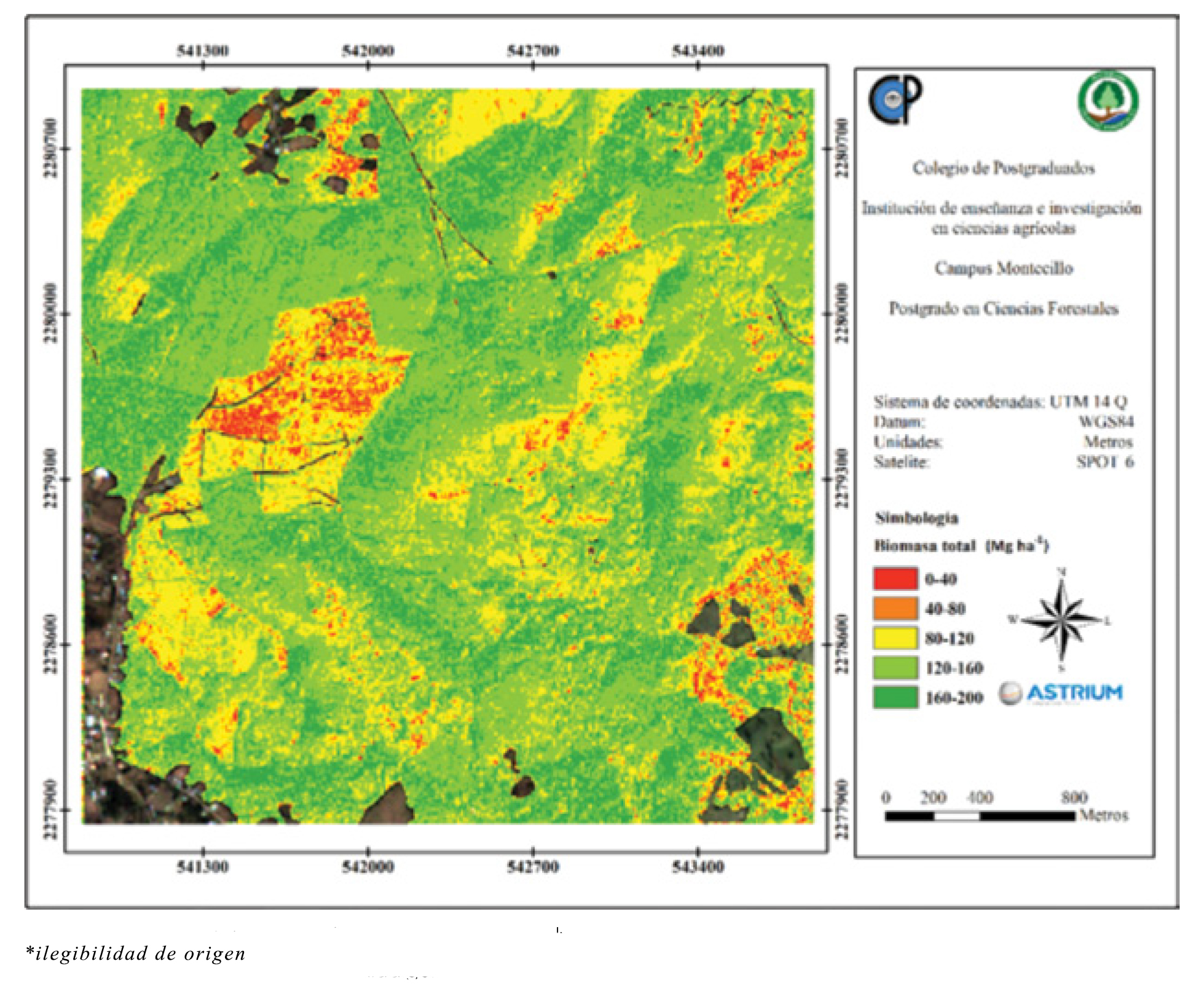
Figure 4 Total biomass of Pinus patula Schiede ex Schltdl. & Cham. under timber management in Zacualtipán, Hidalgo, estimated using multiple linear regression.
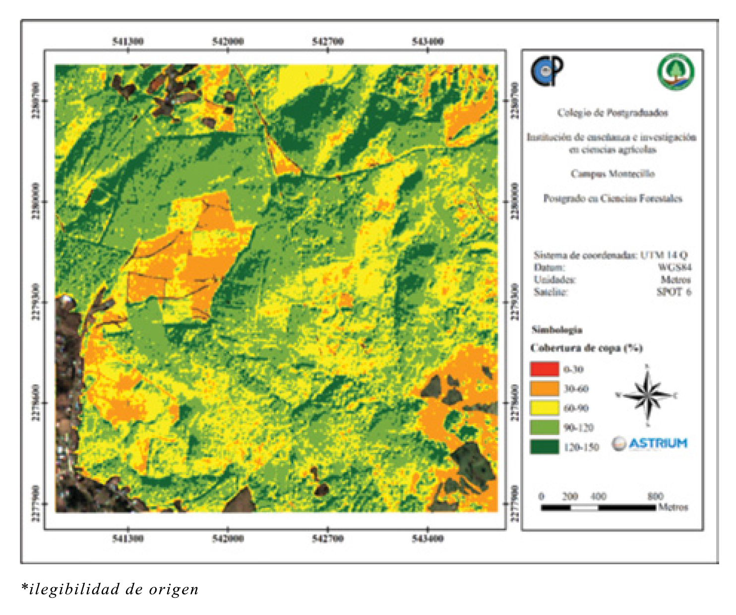
Figure 5 Crown cover of Pinus patula Schiede ex Schltdl. & Cham. under timber management in Zacualtipán, Hidalgo, estimated using multiple linear regression.

Figure 6 Volume of Pinus patula Schiede ex Schltdl. & Cham. under timber management in Zacualtipán, Hidalgo, estimated using multiple linear regression.

Conclusions
The spectral variable of the SPOT-6 sensor that had the highest correlation with most variables of interest (basal area, total biomass, crown cover and volume) was the near infrared band. This is a constant independent variable in regression models adjusted for the estimation of those variables. The leaf area index has a higher correlation with the green band.
The crown cover is the variable with the lowest R2 adj. The total inventories carried out with ratio and regression estimators are located within the confidence interval of the traditional inventory; their results are very reliable and more accurate than those of the traditional inventory.
The regression estimator has a precision interval of 4.8 to 6.9 % for all the assessed variables, while the traditional inventory has a value of 6.5 to 9.3 %. The inventory assisted by spectral data allows generating maps that show the spatial variation of the variable of interest in detail, as well as estimating values for areas where no in-field sampling is carried out.
Acknowledgements
The authors would like to express their gratitude to the Forestry Service of the Department of Agriculture of the United States of America for the funding provided through the Northern Research Station and the Sustainable Landscape Program of the U.S. Agency for International Development. Also, for the support received from Antonia Macedo Cruz, PhD, as manager of the satellite images of the SPOT-6 sensor and, of course, to the Estación de Recepción México Nueva Generación, ERMEX NG) (Reception Station Mexico New Generation) for the SPOT images used in this study
REFERENCES
Aguirre-Salado, C. A., J. R. Valdez-Lazalde, G. Ángeles-Pérez, H. M. de los Santos-Posadas, y A. I. Aguirre-Salado. 2011. Mapeo del índice de área foliar y cobertura arbórea mediante fotografía hemisférica y datos Spot 5 HRG: regresión y k-nn. Agrociencia 45: 105-119. [ Links ]
Aguirre-Salado, C. A., J. R. Valdez-Lazalde, G. Ángeles-Pérez, H. M. de los Santos-Posadas, R. Haapanen, y A. I. Aguirre-Salado. 2009. Mapeo de carbono arbóreo aéreo en bosques manejados de pino patula en Hidalgo, México. Agrociencia43: 209-220. [ Links ]
Ángeles-Pérez, G., C. Wayson, R. Birdsey, J. R. Valdez-Lazalde, H. M. de los Santos-Posadas y F.O. Plascencia-Escalante. 2012. Sitio intensivo de monitoreo de flujos de CO2 a largo plazo en bosques bajo manejo en el centro de México. In: Paz, F. y R. M. Cuevas (eds.). Estado actual del conocimiento del ciclo del carbono y sus interacciones en México: Síntesis 2011. Programa Mexicano del Carbono, Universidad Autónoma del Estado de México e Instituto Nacional de Ecología. Texcoco, Edo. de Méx. México. pp. 2-797. [ Links ]
Astrium. 2013. SPOT 6 & SPOT 7 Imagery User Guide. Toulouse, France. 120p. [ Links ]
Cano M., E. E., A. Velázquez M., J. J. Vargas H., C. Rodríguez F. y A. M. Fierros G. 2006. Área foliar específica en Pinus patula: efecto del tamaño del árbol, edad del follaje y posición en la copa. Agrociencia30: 117-122. [ Links ]
Chuvieco, E. 1995. Fundamentos de teledetección espacial. Ed. Ediciones Rialp. 2a edición. Madrid, España. 224 p. [ Links ]
Comisión Nacional Forestal (Conafor). 2011. Inventario nacional forestal y de suelos: Manual y procedimientos para el muestreo de campo, Re-muestreo 2011. México, D.F., México. 141p. [ Links ]
Cruz-Leyva, I. A., J. R. Valdez-Lazalde, G. Ángeles-Pérez y H. M. de los Santos-Posadas. 2010. Modelación espacial de área basal y volumen de madera en bosques manejados de Pinus patula y P. teocote en el ejido Atopixco, Hidalgo. Madera y Bosques 16(3): 75-97. [ Links ]
Cruz M., Z. 2007. Sistema de ecuaciones para estimación y partición de biomasa aérea en Atopixco, Zacualtipán, Hidalgo, México. Tesis de Maestría en Ciencias. DICIFO. Universidad Autónoma de Chapingo. Chapingo, Edo. de Méx., México. 50p. [ Links ]
INAFED (Instituto para el Federalismo y el Desarrollo Municipal). 2015. Secretaría de Gobernación. Enciclopedia de los municipios de México (EMM). Estado de Hidalgo: Zacualtipán de los Ángeles. Página web. http:// www.inafed.gob.mx/work/enciclopedia/EMM13hidalgo/index.html . (16 de marzo de 2015). [ Links ]
Jensen, J. R. 2007. Remote Sensing of the Environment: An Earth Resource Perspective. Prentice Hall. Second Edition. Upper Saddle River, NJ, USA. 592p. [ Links ]
Figueroa N., C. M., G. Ángeles P., A. Velázquez M., y H. M. de los Santos P. 2010. Estimación de Biomasa en un bosque bajo manejo de Pinus patula Schltdl. et Cham. en Zacualtipán, Hidalgo. Revista Mexicana de Ciencias Forestales 1(1): 105-112. [ Links ]
Hawbaker, T. J., T. Gobakken, A. Lesak, E. Tromborg, K. Contrucci and V. Radeloff. 2010. Light Detection and Ranging based measures of mixed hardwood forest structure. Forest Science 56(3): 313-326. [ Links ]
Merem, E. C. and Y. A. Twumasi. 2008. Using geospatial information technology in natural resources management: the case of urban land management in West Africa. Sensors 8: 607-619. [ Links ]
Muñoz-Ruiz, M. A., J. R. Valdez-Lazalde, H. M. de los Santos-Posadas, G. Ángeles-Pérez, y A. I. Monterroso-Rivas. 2014. Inventario y mapeo del bosque templado de Hidalgo, México mediante datos del satélite SPOT y de campo. Agrociencia48: 847-862. [ Links ]
Ortiz-Reyes, A. D., J. R. Valdez-Lazalde, H. M. de los Santos-Posadas, G. Ángeles-Pérez, F. Paz-Pellat, y T. Martínez-Trinidad. 2015. Inventario y cartografía de variables del bosque con datos derivados de LiDAR: comparación de métodos. Madera y Bosque 21(3): 111-128. [ Links ]
Scheaffer, L. R., W. Mendenhall and L. Ott. 1986. Elementary survey sampling. PWS Publishers. Boston, MA, USA. 320p. [ Links ]
Soriano-Luna, M. de los A., G. Ángeles-Pérez, T. Martínez-Trinidad, F. O. Plascencia-Escalante, y R. Razo-Zárate. 2015. Estimación de biomasa aérea por componentes estructurales en Zacualtipán, Hidalgo, México. Agrociencia 49: 423-438. [ Links ]
Tanaka, S., T. Takahashi, T. Nishizono, F. Kitahara, H. Saito, T. Iehara, E. Kodani, and Y. Awaya. 2014. Stand volume estimation using the k-NN technique combined with forest inventory data, satellite image data and additional feature variables. Remote Sensing 7: 378-394. [ Links ]
Valdez-Lazalde, J. R., M. de J. González-Guillén, y H. M. de los Santos-Posadas. 2006. Estimación de cobertura arbórea mediante imágenes satelitales multiespectrales de alta resolución. Agrociencia 40: 383-394. [ Links ]
Velasco L., S., O. Champo J., Ma. L. España B., y F. Baret. 2010. Estimación del índice de área foliar en la reserva de la biósfera mariposa monarca. Revista Fitotecnia Mexicana 33(2): 169-174 [ Links ]
Received: November 13, 2016; Accepted: February 06, 2017
 Este es un artículo publicado en acceso abierto bajo una licencia Creative Commons
