a) Physical location and characteristics of the study área

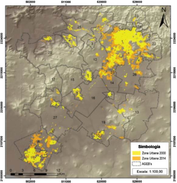
The study area is located in the south of the state of Hidalgo and comprises the municipalities of Pachuca, Mineral de la Reforma, Zapotlán de Juárez, Villa de Tezontepec, Tolcayuca, Tizayuca and part of San Agustín Tlaxiaca and Zempoala (Figure 1), with a total surface area of 964.45 km2 (Figure 1).

Figure 1 Location of the Pachuca-Tizayuca corridor. 

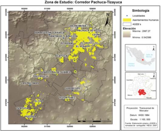
In physiographical terms, the region is part of the Transversal Neovolcanic Axis province, with topoforms that include mountain chains, plains and rolling hills (^{Inegi, 2014}). Most of the mountain chain area is located to the north, and a small part of it is south of the area (^{Inegi, 2014}). That system is formed by andesitic and dacitic volcanic rocks corresponding to the Tertiary period (^{SGM, 2007}). The rolling hills are situated in the northeast (^{Inegi, 2014}), in Mineral de la Reforma; they are made up of andesite, dacite and dacitic tuff. The plains are located in the central and southern portion, coinciding with the majority of the human settlements; they have a NNE- SSW orientation and are constituted by volcano-sedimentary material from the surrounding sierra and rolling hills (^{SGM, 2007}). They are part of the hydrographic area of the Pánuco river (EH26) and belong to the basin of the Moctezuma river. The predominant climate is semi-dry temperate and sub-humid temperate (^{Inegi, 2008}).

The vegetation is represented by xerophyllic shrubs and induced grasslands. The former are distributed in the periphery of the valley, mainly on the Cubitos mountain, and include species in the NOM-059-SEMARNAT-2010 norm, such as Coryphantha werdemannii Boed., Turbinicarpus pseudomacrochele ( Backeb.) Buxb. & Backeb., considered in the Endangered Species category; Astrophytum ornatum (DC) Britton & Rose, Cephalocereus seniles (Haw.) Pfeiff., Ferocactus stainesii (Salm-Dyck) Britton & Rose var. pilosus (Galeotti ex Salm- Dyck) Backeb., Mammillaria klissingiana Boed., Mammillaria longimamma DC., Mammillaria zephyranthoides Scheidw., classified as Threatened, and Coryphantha durangensis (Runge ex Schum.) Britton & Rose, Coryphantha radians Britton & Rose, Coryphantha retusa Britton & Rose, Echinocactus platyacanthus Link & Otto, Echinocereus pulchellus (Mart.) K. Schum., Ferocactus histrix (DC.) G.E. Linds., Stenocactus coptonogonus (Lem.) A. Berger ex A. W. Hill, Thelocactus leucacanthus (Zucc. Ex Pfeiff.) Britton & Rose, under Special Protection (^{Zuria and Rendón, 2010}).

The forest vegetation is distributed in the north of the study area, within the El Chico National Park, and consists of Sacred fir (Abies religiosa (Kunth) Schltdl. & Cham.), Mexican juniper (Juniperus monticola Martínez) and, to a lesser extent, oak (Quercus spp.) forests. According to the NOM-059- SEMARNAT-2010 norm, Pseudotsuga macrolepis, Taxus globosa and Litsea glaucescens are classified as Endangered, and Fucrea bendinghaussii, as Threatened (Conanp, 2005).

In order to determine the impact of rapid urbanization on the natural ecosystem adjoining the Pachuca-Tizayuca corridor, territorial units were established upon the basis of the Rural Basic Statistical Geographical Area (AGEB) defined by ^{Inegi (2007)}. This division was selected because it reflects homogenous socioeconomic characteristics, it takes into account municipal boundaries, and the size of the areas allows a more detailed analysis of the territory than the municipal level.

The ratio of the urban sprawl to the difference between the vegetation indices (ΔVI) and was compared to the distance to human settlements (DU); for this purpose, the following actions were carried out: a) the urbanized area was determined for the years 2000 and 2014; b) the climatic context of the area was analyzed to evaluate the comparability between those years; c) the VIs and the differences between the two years ΔVI_00-14 were estimated, and the urban sprawl for was compared between the AGEBs, and d) the correlations between the ΔVI and the DU were determined.

b) Estimation of the urban sprawl between 2000 and 2014

Three multispectral Landsat ETM and OLI images -Path-Row 26/46- of February 2000 and 2014 from the website of the United States Geographical Service (USGS), with a pixel resolution of 30 m on a side, were used. They were geometrically corrected using control points obtained from orthophotos (scale 1:75 000). Next, the radiometric (Chander et al., 2009) and atmospheric calibrations were carried out using the ENVI 5.1 software and the FLAASH (Fast Line-of- sight Atmospheric Analysis of Spectral Hypercubes) correction developed by ^{Kruse (2004)}, as proposed by ^{Arias et al. (2015)}, in order to convert the digital levels into radiance values and, subsequently, to normalized reflectance values, which can be contrasted between different periods (Hantson et al., 2011).

The supervised classification was based on the 80 areas of training that were known or had been verified in the field. This is a widely used method to classify the cover and land use in Mexico (García-Mora and Mas, 2008; Figueroa-Jáuregui et al., 201), based on the establishment of reflectance values which the classification groups by maximum plausibility using the IDRI Taiga software, whose performance in the detection and modeling of the change of land use is very good, unlike other techniques (^{Mas et al., 2014}).

Its effectiveness was evaluated using confusion matrices, based on random samples with 400 and 300 verification points for 2000 and 2014, respectively, since large populations (>10 000) do not require a sample above 100 (^{Mas et al., 2003}).

The SAMPLE module of the IDRISI software was utilized, taking its ground truth as a basis for field visits as well as Google Earth images and orthophotos (^{Inegi, 1999}). The omission and commission errors were estimated for 10 classes of land cover: water, secondary forest, conifer forest, fallow land, eroded areas/areas without vegetation, urban area, cultivated land, open and altered shrublands, dense and healthy shrublands, and natural and induced grasslands. The standard deviation (≤ 0.05) was estimated based on the sample size and on the percentage of confidence interval, as recommended by ^{Mas et al. (2003)}. The classified images were filtered and converted into polygons in order to estimate the urban areas of 2000 and 2014 and their differences.

c) Description of the climatic context of the area

This work is part of a series of evaluations carried out during the same period -e.g. one month (^{Morawitz et al., 2006}) or more (^{Levin, 2015})- in different years in order to measure the variations in the vegetation beyond seasonality (Benliay and Altuntaş, 2014). For this reason, the climatic tendencies of average annual precipitation and temperature parameters of the climatological stations within and on the edges of the study area were found and their location is described in Table 1.

Table 1 Climatological stations utilized to describe the climatic context of the area. 

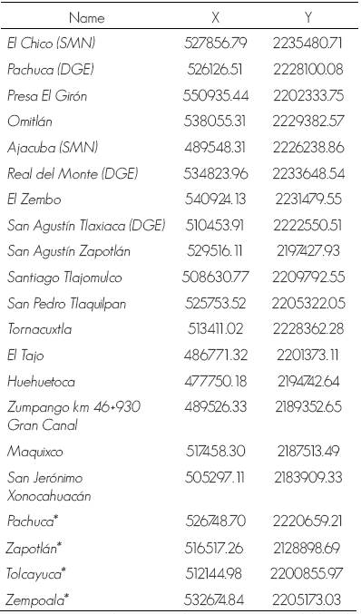
SMN= Servicio Meteorológico Nacional; DGE=Dirección General del Estado.

*Climate stations of INIFAP

The data from the stations between 1980 and 2014 were used. Based on their variances, it was determined whether or not the conditions of precipitation and temperature in the years 2000 and 2014 are comparable, since these have been shown to be the factors that most influence changes in the vegetation (^{Mao et al., 2012}). Thus, the effect of the changes in the vegetation caused by the climatic factors in the correlation between ΔVI_00-14 and DU are considered.

d) Calculation of the difference between the vegetation indices in 2000 and 2014 and comparison between urbanization in each AGEB

Different VIs were calculated for the whole study area with the equations described in Table 2, using the ENVI 5.1 software.

Table 2 Vegetation indices and their application in the study area. 

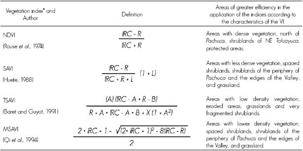
*NDVI = Normalized Difference Vegetation Index; SAVI = Soil Adjusted Vegetation Index; TSAVI = Transformed Soil Adjusted Vegetation Index, MSAVI = Modified Soil Adjusted Vegetation Index; IRC = Near infrared band; R = Red band; L = Parameter consisting in a soil-adjusted constant, and X allowing to minimize the maximum soil effect.

For the TSAVI index, the soil line was defined according to Eastman (2009), who describes how to estimate the slope and the intercept of the values of the soil line based on a regression between the values of the pixels on the naked soil in relation to the values of the red or infrared band.

Once the indices were calculated, the main differences between the VIs were estimated, using the raster calculation for the evaluated years. The rasters resulting from the difference between the VIs (NDVI, SAVI, MSAVI, TSAVI) in the period 2000 and 2014 were denominated ΔVI_00-14.

The mean values of the ΔVI_00-14 for each AGEB were estimated and compared to the proportion of urbanized surface area in each AGEB by means of charts in order to determine whether or not there is a relationship between the increase in urbanization and the ΔVIs_00-14 (^{Morawitz et al., 2006}; Dhorde et al., 2012).

e) Spatial correlations between the VIs and the distance to the urban áreas

The ΔVI vs. DU correlation was estimated using a bivariate spatial regression, with the REGRESS command of the IDRISI Taiga software (Eastman, 2009). In order to measure it, a Boolean raster file was generated for each analysis unit (AGEB), and 10 % of the pixels were randomly extracted from each. In order to rule out the existence of a self-correlation, "Moran's I" test was applied, using the SELF CHECK command of the same software.

Next, the AGEBs in which the ΔVI has the highest correlation to DU were identified, determining the sign of this correlation, in which the dependent variable is the DIV and the independent variable is DU.

a) Supervised classification

It consists in differentiating the urban area from other types of vegetal covers. In the case of the classification for the year 2000, the average omission and commission errors were of 0.17 and 0.15, respectively. Table 3 summarizes the reliability data for the entire confusion matrix. The average value was 0.83, and therefore the defined urban areas are reliable.

Table 3 User's and producer's reliability for the soil cover categories classified for 2000 and 2014. 

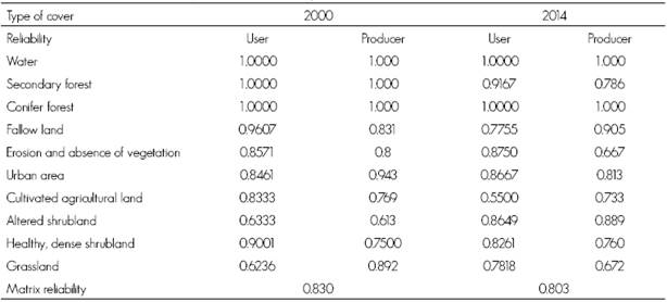
For the year 2014, the classification had an omission error of 0.13 and a commission error of 0.14. The average reliability of the classification was 80.3 % (Table 3). Based on these values, the urban area has grown by 51 % in the municipality of Pachuca, by 138 % in Mineral de la Reforma, and by 41 %, 13 % and 88 % in Villa de Tezontepec, Tolcayuca and Tizayuca, respectively.

Figure 2 shows the map of the growth of the urban sprawl in the study area between the years 2000 and 2014.

Figure 2 Differences in the urban soil between 2000 and 2014 estimated with supervised classification. The map shows the division by Rural AGEBs. 

b) The years 2000 and 2014 within the climatic context of the area

The mean temperature was 14.82 ± 0.42 °C. A tendency ranging between 14.6 °C, in 1980, and 15.0 °C, in 2014, was observed; therefore, in the last 30 years there has been a warming of 0.4 °C (Figure 3).

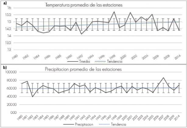
Source: Temperature (a) and precipitation (b) data from the existing climate stations of the NMS from 1980 to 2009. Except for 2014, which is an average of the climate stations of INIFAP, since the NMS only has information available for the period from 1980 to 2010.

Figure 3 Temperature (a) and precipitation (b) data from annual measurements through 30 years (1980-2014). 

During the studied period, the mean temperature in the year 2000 was 14.8 °C for a variation of under 0.2 °C; it is therefore assumed that this variation did not affect the vegetation.

The mean precipitation value was 604 ± 95 mm, with a high standard deviation; this is indicative of the most disperse, unpredictable behavior of this parameter. For example, in the year 2007 there was an extreme event with high precipitations, a factor which may have influenced the results of the estimated ΔVls_00-14.

c) Preliminary assessment of ΔVIs adjoining urbanization in each AGEB

The estimated ΔVIs show in which of the 27 AGEBs there was a coincidence with the growth of urbanization, as well as the changes in each of the estimated ΔVIs between the years 2000 and 2014 and their sign (Figure 4). The units with greatest impact on the vegetation were AGEBs 4, 7, 1, 14, 18, 25 and 26; of these, only AGEB 4 suffered a negative impact.

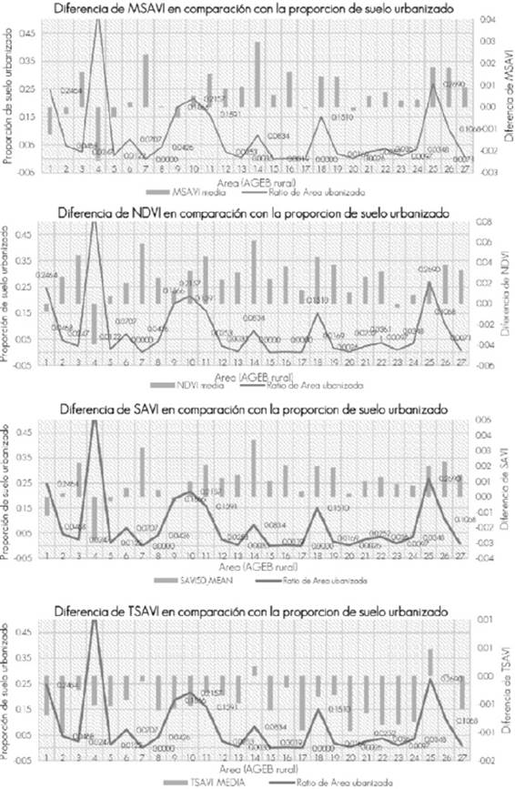
Figure 4 Positive and negative differences between the VIs compared to the urbanized soil. (AGEB on the X-axis. Proportion of urbanized soil (U/UN ratios) by AGEB and ΔVIs on the Y-axis). 

The urban sprawl was observed to have grown considerably in 10 AGEBs; in these cases, the DIV was not always negative.

Unfavorable relationships between the ΔVI and the U/NU urbanization ratio. In the AGEBs in which the urbanized area grew, the ΔVI was negative. These areas correspond in general to the settlements, towns and cities (Pachuca, AGEB 1; the Mineral de la Reforma residential developments, AGEB 4, and Tizayuca, AGEB 9), which have spread over the native vegetation or are due to the use of the shrublands and grasslands, as in the municipality of Zapotlán de Juárez (AGEB 6, TSAVI).

Favorable relationships between the ΔVI and the U/NU urbanization ratio. These occurred in the AGEBs whose cultivation areas have expanded and which have positive ΔVIs, despite urbanization. This is evident, especially in the southern residential developments of the Pachuca municipality (AGEB 25) and of Mineral de la Reforma (AGEB 26), and, to a lesser degree, in Jagüey de Téllez (AGEB 14), El Cid (AGEB 18), Villa de Tezontepec (AGEB 10) and Tizayuca-Huizila (AGEB 11).

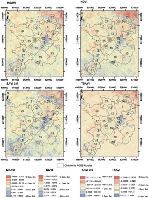
Figure 5 includes the maps with the location of the AGEBs for each estimated ΔVI. Increases in the ΔVIs -e.g. those sites where the vegetation has recuperated- are highlighted in blue; ΔVI losses are highlighted in red.

Prepared based on the determined VIs and modifications to the soil, classified by standard deviation.

Figure 5: Positive and negative differences between the VIs by Rural AGEB. 

d) Spatial correlations between the ΔVIs and the DU distance to the urban areas

The correlation between the ΔVIs and the DU was estimated for each analysis unit (AGEB). The self-correlation in each was ruled out using Moran's I test, which gave as a result an average value of 0.07. This means that the proximity of the extracted pixels did not produce a specification error.

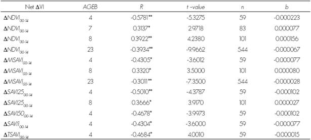
Table 4 shows the linear regression parameters of the correlations that turned out to be significant and have higher R-values for the net values of ΔVI vs. DU.

Table 4 Parameters of significant correlations ΔVI vs. DU in AGEB. 

*Significance level p< 0.05,

** Significance level p < 0.01, (Without asterisk=Not significant)

R = Linear correlation coefficient; t-value = Student's t; n = Number of pixels; β= Slope of the linear regression line.

REFERENCES

Arias, H. A., R. M. Zamora y C. V. Bolaños. 2015. Metodología para la corrección atmosférica de imágenes Aster, RapidEye, Spot 2 y Landsat 8 con el módulo FLAASH del software ENVI. Revista Geográfica de América Central:39-60. [ Links ]
Bannari, A., D. Morin and A. Huete. 1995. A review of vegetation indices. Remote Sensing Reviews:95-120. [ Links ]
Baret, F. and G. Guyot. 1991. Potentials and limits of vegetation indices for LAI and APAR assessment. Remote Sensing of Environment 35(2-3): 161-173. [ Links ]
Huete, A. R. 1988. A soil-adjusted vegetation index (SAVI). Remote sensing of environment 25: 295-309. [ Links ]
Instituto Nacional de Estadística, Geografía e Informática (Inegi). 1999. Ortofotos digitales. Fuente: fotografías aéreas escala 1:75 000. Proyección: UTM. Datum: ITRF92. Elipsoide: GRS 80. Dimensiones del pixel X,Y: 1.5 metros. Productos geográficos básicos digitales. Instituto Nacional de Estadística Geografía e Informática. México, D.F., México. s/p. [ Links ]
Instituto Nacional de Estadística, Geografía e Informática (Inegi). 2007. Conjunto de datos vectoriales de áreas geoestadísticas básicas rurales. Instituto Nacional de Estadística y geografía. Aguascalientes, Ags., México. s/p. [ Links ]
Instituto Nacional de Estadística, Geografía e Informática (Inegi). 2008. Conjunto de datos vectoriales de Unidades Climáticas Escala 1:1 000 000. Instituto Nacional de Estadística y Geografía. Aguascalientes, Ags., México. s/p. [ Links ]
Instituto Nacional de Estadística, Geografía e Informática (Inegi). 2014. Anuario estadístico y geografico de Hidalgo 2013. Instituto Nacional de Estadística y Geografía. Aguascalientes, Ags., México. 573 p. [ Links ]
Jenerette, G. D., S. L. Harlan, A. Brazel, N. Jones, L. Larsen and W. L. Stefanov. 2007. Regional relationships between surface temperature, vegetation, and human settlement in a rapidly urbanizing ecosystem. Landscape Ecology 22:353-365. [ Links ]
Kruse, F. A., 2004. Comparison of ATREM, ACORN, and FLAASH atmospheric corrections using low-altitude AVIRIS data of Boulder, CO. In: Green, R. O. (ed.). Quiénes Summaries of 13th JPL Airborne Geoscience Workshop, Jet Propulsion Lab. Pasadena, CA. http://trs-new.jpl.nasa.gov/dspace/bitstream/2014/38724/1/05-3.pdf (30 de noviembre de 2015). [ Links ]
Levin, N. 2015. Human factors explain the majority of MODIS-derived trends in vegetation cover in Israel: a densely populated country in the eastern Mediterranean. Regional Environmental Change DOI.10.100.7/s10113-015-0848-4. [ Links ]
Li, G. Y., S. Chen, Y. Yan and C. Yu. 2014. Effects of Urbanization on Vegetation Degradation in the Yangtze River Delta of China: Assessment Based on SPOT-VGT NDVI. Journal of Urban Planning Development 141(4): 10.1061/(ASCE)UP.1943-5444.0000249. [ Links ]
Mao, D., Z. Wang, L. Luo and C. Ren. 2012. Integrating AVHRR and MODIS data to monitor NDVI changes and their relationships with climatic parameters in Northeast China. International Journal of Applied Earth Observation and Geoinformation 18:528-536. [ Links ]
Martin, C. A., P. S. Warren and A. P. Kinzig. 2004. Neighborhood socioeconomic status is a useful predictor of perennial landscape vegetation in residential neighborhoods and embedded small parks of Phoenix, AZ. Landscape and Urban Planning 69: 355-368. [ Links ]
Mas, J. F., J. R. Díaz-Gallegos y A. Pérez-Vega. 2003. Evaluación de la confiabilidad temática de mapas o de imágenes clasificadas: una revisión. Investigaciones Geográficas 51: 53-72. [ Links ]
Mas, J. F., M. Kolb, M. Paegelow, M. T. Camacho O. and T. Houet. 2014. Inductive pattern-based land use/cover change models: A comparison of four software packages. Environmental Modelling & Software 51: 94-111. [ Links ]
Meneses-Tovar, C. L. 2011. El índice normalizado diferencial de la vegetación como indicador de la degradación del bosque. Unasylva 238(62):39-46. [ Links ]
Mennis, J., 2006. Socioeconomic-Vegetation Relationships in Urban, Residential Land. Photogrammetric Engineering & Remote Sensing 72: 911-921. [ Links ]
Morawitz, D., T. Blewett, A. Cohen and M. Alberti. 2006. Using NDVI to Assess Vegetative Land Cover Change in Central Puget Sound. Environmental Monitoring and Assessment 114: 85-106. [ Links ]
Pérez-Morales, J. A. 2014. Índice de degradación de la vegetación sometida a manejo forestal en el sur de Nuevo León, México. Tesis de Maestría. Universidad Autónoma de Nuevo León. Nuevo León, N.L., México. 68 p. [ Links ]
Pineda-Jaimes, N., J. Bosque S., M. Gómez D. y W. Plata R. 2009. Análisis de cambio del uso del suelo en el Estado de México mediante sistemas de información geográfica y técnicas de regresión multivariantes. Una aproximación a los procesos de deforestación. Investigaciones Geográficas , Boletín del Instituto de Geografía, UNAM 69:33-52. [ Links ]
Qi, J., A. Chehbouni, A. Huete , Y. Kerr and S. Sorooshian. 1994. A modified soil adjusted vegetation index. Remote sensing of environment 48: 119-126. [ Links ]
Rouse, J. W., H. R. Haas, D. W. Deering, J. A. Schell and J. C. Harlan. 1974. Monitoring the vernal advancement and retrogradation (green wave effect) of natural vegetation. NASA/GSFC. Greenbelt, MD, USA. 371 p. [ Links ]
Servicio Geológico Mexicano (SGM). 2007. Carta Geológico-Minera f14-11. Estado de Hidalgo. Escala 1:250 000. Mexico. Secretaria de Economía, México, D.F., México. s/p. [ Links ]
Sun, J., X. Wang, A. Chen, Y. Ma, M. Cui and S. Piao. 2011. NDVI indicated characteristics of vegetation cover change in China's metropolises over the last three decades. Environmental Monitoring and Assessment 179:1-14. [ Links ]
Torres, E., G. Linares, M. G. Tenorio, R. Peña, R. Castelán y A. Rodríguez. 2014. Índices de vegetación y Uso de Suelo en la Región Terrestre Prioritaria 105: Cuetzalan, México. Revista Iberoamericana de Ciencias 1(3):101-112. [ Links ]
Wessels, K. J., S. D. Prince, J. Malherbe, J. Small, P. E. Frost and D. VanZyl. 2007. Can human-induced land degradation be distinguished from the effects of rainfall variability? A case study in South Africa. Journal of Arid Environments 68: 271-297. [ Links ]
Zuria, I. and H. G. Rendón. 2010. Notes on the breeding biology of common resident birds in an urbanized area of Hidalgo, Mexico. Huitzil 11(1): 35-41. [ Links ]
Este es un artículo publicado en acceso abierto bajo una licencia Creative Commons