


Serviços Personalizados
Journal
Artigo
 texto em
  Inglês (pdf)
 Artigo em XML
 Referências do artigo
 Enviar este artigo por email
Indicadores
-
 Citado por SciELO
 -
 Acessos
Links relacionados
-
 Similares em
SciELO
Similares em
SciELO
Compartilhar

 Permalink
Revista mexicana de ciencias pecuarias
versão On-line ISSN 2448-6698versão impressa ISSN 2007-1124
Rev. mex. de cienc. pecuarias vol.14 no.2 Mérida Abr./Jun. 2023 Epub 26-Jun-2023
https://doi.org/10.22319/rmcp.v14i2.6250
Articles
Genetic structure and variability in American bison (Bison bison) in Mexico
a Universidad Autónoma de Chihuahua. Facultad de Zootecnia y Ecología. Periférico Francisco R. Almada Km. 1, CP 31453. Chihuahua, Chihuahua, México.
b Universidad Autónoma de Baja California. Instituto de Ingeniería. Baja California, México.
c Fondo Cuenca Los Ojos, Rancho El Uno. Chihuahua, México.
d Fondo Mexicano para Conservación de la Naturaleza. Chihuahua, México.
Controlling for genetic variables to managing conservation populations. Single nucleotide polymorphism (SNP) genetic markers were used to analyze genetic structure and variability in an American bison population in the state of Chihuahua, Mexico. A total of 174 individuals were sampled and analysis done of 42,366 SNP distributed in 29 chromosomes. Estimates were done of expected (He) and observed (Ho) heterozygosity, polymorphic information content (PIC), the fixation index (FST), the Shannon index (SI), linkage disequilibrium (LD), kinship relationships (Rij; %), and effective population size (Ne). A genetic structure analysis was run to infer how many lines or genomes (k) define the studied population. A panel with 2,135 polymorphic SNPs was identified and selected, with an average of 74 SNP per chromosome. In the exclusion process, 84.5 % were monomorphic, 8.5 % had a usable percentage less than 90 %, 6.3 % had a minor allele frequency less than 0.01 and 0.70 % exhibited Hardy-Weinberg disequilibrium (P<0.05). Estimated values were 0.30 for the SI, 0.187 for Ho, 0.182 for He, -0.029 for the FST, and 0.152 for PIC. Of the 15,051 Rij estimates generated, the average value was 7.6 %, and 45.1 % were equal to zero. The Ne was 12.5, indicating a possible increase of 4 % in consanguinity per generation. Three genetic lines were identified (proportions = 0.730, 0.157 and 0.113), and, given the study population’s origin, are probably associated with natural selection or genetic drift. Genetic variability, as well as Rij levels, must be considered in conservation schemes.
Key words Heterozygosis; Genetic resources; Effective population size; Consanguinity; Conservation; SNP
Los objetivos fueron analizar la estructura y variabilidad genética del bisonte americano con marcadores genéticos de tipo SNP. Se muestrearon 174 bisontes y se analizaron 42,366 SNP distribuidos en los 29 cromosomas. Se estimó la heterocigosis esperada (He) y observada (Ho), contenido de información polimórfica (CIP), índice de fijación (FIS), índice de Shannon (IS), desequilibrio de ligamiento y relación de parentesco (Rij; %), así como el tamaño efectivo de población (Ne). Se realizó un análisis de estructura genética para inferir cuántas líneas o genomas (k) definen la población. Se identificó y seleccionó un panel con 2,135 SNP polimórficos, con un promedio de 74 SNP por cromosoma. En el proceso de exclusión, 84.5 % fueron monomórficos, 8.5 % con porcentaje de usables menor a 90 %, 6.3 % con frecuencia del alelo menor inferior a 0.01 y 0.70 % por desequilibrio Hardy-Weinberg (P<0.05). Las estimaciones de IS, Ho, He, FIS y CIP fueron de 0.30, 0.187, 0.182, -0.029 y 0.152, respectivamente. Se generaron 15,051 estimaciones de Rij, el valor promedio de éstas fue 7.6 %, y el 45.1 % de ellas fue igual a cero. El Ne fue de 12.5, señalando un posible incremento de consanguinidad por generación de 4 %. Se identificaron tres líneas genéticas, con proporciones de 0.730, 0.157 y 0.113; dado el origen de la población, se asocian a selección natural o deriva genética. La variabilidad genética, así como los niveles de la Rij, se deben de considerar en esquemas de conservación.
Palabras clave Heterocigosis; Recursos genéticos; Tamaño efectivo de población; Consanguinidad; Conservación; SNP
Introduction
The Bison genus (bison) is native to Asia and central Europe, but migrated to the American continent via the steppe bison (Bison priscus) and the giant bison (Bison latifrons). Current populations of American bison (AB; Bison bison) are the product of adaptation, evolution and natural selection; there are two allopatric subspecies, the plains bison (Bison bison bison) and the mountain bison (Bison bison athabascae). Historical and archaeological data suggest that the AB developed on the North American prairies, with estimated populations as high as 60 million individuals. During the 19th Century, bison hunting for food and hides decimated the population, bringing it near extinction1,2,3,4.
In Mexico, there are historical accounts of AB in the states of Chihuahua, Coahuila, Durango and Sonora; the Janos-Hidalgo herd was a transboundary herd that moved between Chihuahua and New Mexico5,6. There is currently a conservation herd at El Uno Ranch, in the Janos Biosphere Reserve (Chihuahua, Mexico), which was created with 23 individuals from Wind Cave National Park in the United States7. As a genetic resource, the AB exhibits the time and space components, as well as use and option values of biodiversity. The time and space components are determined by evolution and changes in species richness, relative abundance and dominance. The use value consists of the benefits provided by the resource, and the option value is defined by a genetic resource’s role in or contribution to ecosystem stability8,9.
Population biodiversity is the product of adaptation to and integration into ecosystems driven by evolutionary forces and population genetics (e.g., natural selection, genetic drift and migration). Genetic diversity is a component of biodiversity and comprises differences in heritable genetic material. Genetic variability is a measure of genotype differentiation as a function of population size and the criteria used to define inheritance of genetic material. Determined by its evolutionary history, a population’s genetic structure expresses the genetic diversity it harbors and this is distributed within the population. Loss of genetic diversity is the main challenge in at-risk populations, and is therefore a vital concept in the design of conservation schemes10,11. The present study objective was to analyze the genetic structure and variability of the AB herd at El Uno Ranch using simple nucleotide polymorphism (SNP) genetic markers.
Material and methods
The AB herd at El Uno Ranch exists in a wild environment with almost no human contact, and is isolated and protected from populations of other bovids or other species that could alter its normal development. All ranch personnel are specialized and facilities are exclusively for managing the herd. A herd census and identification is done annually. For the present study, 174 animals (80 % of the total herd) were sampled: 102 females and 72 males born in 2012. Blood deposited on specialized cards in the GeneSeek Laboratory of Neogen® Corporation was used for DNA extraction. Analyses were done of 42,366 SNP genotypes distributed in 29 chromosomes and defined in the GGP Bovine 50K chip. During editing, loci were discarded if they had a usable percentage (UP) <90 %, were monomorphic, had a minor allele frequency (MAF) <0.01 and/or were in Hardy-Weinberg disequilibrium (HW; P<0.05).
After editing, the SNPs panel was used to estimate six genetic variability indicators: expected heterozygosity (He); observed heterozygosity (Ho); polymorphic information content (PIC); the fixation index (FST); the Shannon index (SI) and linkage disequilibrium (LD)12,13. The LD was evaluated based on the correlation (r2) between haplotype frequencies through loci14. Correlation (r2) values range from zero to one, with values near zero indicating an absence of LD and independent segregation and those near 1 indicating non-random association between loci. The kinship relationship (Rij; %) was estimated using all the sampled individuals and the effective population size (Ne) based on adjusted average r2 via the Waples method14. Estimates of r2 were done using the FSTAT program15; the GenAlex program16 was used to estimate He, Ho, PIC and the FST; the LDNE program17 was used to analyze Ne; and ML-Relate18 was applied to estimate Rij.
Genetic structure was elucidated with the Structure genetic analysis program19. This uses Bayesian grouping to infer the number of lines or genomes (k) within a population by using genetic markers for genotype analysis. The procedure assumes that individuals are of pure ancestry (k= 1) vs. ancestry of two or more lines (k ≠ 1), and proportionally assigns a genome to each line. Use of Bayesian clustering to infer k is derived from the a posteriori probability distribution generated by the Markov Chain-based Monte Carlo method. Five possible lines were evaluated in the present study, and individuals were assigned to them probabilistically. The number of lines (k) that provides the best fit is derived from the logarithmic likelihood of each sampling step, and the maximum or optimal value was obtained with the approach of Evanno et al.20 and the Structure Harvester program21.
Results and discussion
Editing produced a panel with 2,135 identified and selected SNPs (5.04 % yield versus total number of evaluated SNPs), with an average of 74 SNPs per chromosome. A total of 40,231 SNPs were discarded: 84.5 % were monomorphic; 8.5 % by UP<90 %, 6.3 % by MAF<0.01, and 0.70 % by HW in disequilibrium. The panel of selected SNPs had a SI of 0.30, a Ho of 0.187, a He of 0.182, a FST of -0.029, and a PIC of 0.152 (Table 1). The He, Ho and PIC values determine genetic marker viability in genetic variability studies. All SI estimates were nearer zero than one, which is associated with homogeneity in the population and reduces uncertainty when predicting the probability of assignment of an individual to a population. In all the chromosomes FST had values ranging from -0.002 to -0.062. This indicator measures levels of heterozygosis and homozygosis, and produces values between -1 and 1. Positive values indicate a heterozygote deficit and negative ones an excess. Values near zero are a sign of stability in the homozygous/heterozygous relationship. The average Rij value was 7.61 % based on 15,051 estimates from 174 individuals. Within the 0 to 100 % range of this indicator, the present results could be classified into five strata: 45.1 % of the estimates were equal to zero; 14.5 % were from 0.01 to 4.9; 27.3 % from 5.0 to 19.9; 11.8 % from 20.0 to 49.9; and 1.3 % were equal to or greater than 50.0. An individual’s consanguinity (F) is half the Rij of its parents. Estimates of Rij can therefore be used to select subpopulations for reproduction and conservation schemes, with a view to maintaining F levels.
Table 1 Number of SNPs, and genetic variability estimators per chromosome
| Cr | ni | nf | PIC | Ho | He | FST | SI | r2 |
|---|---|---|---|---|---|---|---|---|
| 1 | 2587 | 88 | 0.155 | 0.194 | 0.186 | -0.034 | 0.304 | 0.022 |
| 2 | 2199 | 52 | 0.153 | 0.193 | 0.186 | -0.029 | 0.302 | 0.019 |
| 3 | 2072 | 56 | 0.211 | 0.263 | 0.260 | -0.011 | 0.403 | 0.023 |
| 4 | 1933 | 170 | 0.117 | 0.140 | 0.136 | -0.035 | 0.241 | 0.222 |
| 5 | 2173 | 160 | 0.105 | 0.126 | 0.122 | -0.025 | 0.215 | 0.205 |
| 6 | 2056 | 70 | 0.193 | 0.240 | 0.234 | -0.025 | 0.372 | 0.020 |
| 7 | 1858 | 232 | 0.195 | 0.240 | 0.226 | -0.062 | 0.376 | 0.324 |
| 8 | 1832 | 47 | 0.186 | 0.228 | 0.225 | -0.024 | 0.359 | 0.021 |
| 9 | 1818 | 57 | 0.230 | 0.298 | 0.289 | -0.032 | 0.437 | 0.026 |
| 10 | 1736 | 205 | 0.089 | 0.107 | 0.103 | -0.028 | 0.189 | 0.288 |
| 11 | 1766 | 52 | 0.143 | 0.174 | 0.170 | -0.019 | 0.282 | 0.019 |
| 12 | 1418 | 49 | 0.218 | 0.281 | 0.270 | -0.034 | 0.415 | 0.031 |
| 13 | 1544 | 65 | 0.151 | 0.192 | 0.187 | -0.020 | 0.295 | 0.127 |
| 14 | 1483 | 61 | 0.156 | 0.190 | 0.189 | -0.013 | 0.307 | 0.105 |
| 15 | 1395 | 59 | 0.176 | 0.221 | 0.212 | -0.034 | 0.342 | 0.022 |
| 16 | 1302 | 40 | 0.194 | 0.247 | 0.235 | -0.044 | 0.372 | 0.024 |
| 17 | 1233 | 41 | 0.195 | 0.246 | 0.239 | -0.021 | 0.375 | 0.026 |
| 18 | 1219 | 33 | 0.210 | 0.267 | 0.255 | -0.039 | 0.399 | 0.028 |
| 19 | 1218 | 65 | 0.124 | 0.147 | 0.146 | -0.016 | 0.251 | 0.210 |
| 20 | 1335 | 50 | 0.192 | 0.238 | 0.232 | -0.031 | 0.370 | 0.026 |
| 21 | 1183 | 33 | 0.185 | 0.235 | 0.228 | -0.032 | 0.358 | 0.024 |
| 22 | 1017 | 23 | 0.197 | 0.242 | 0.239 | -0.017 | 0.379 | 0.029 |
| 23 | 943 | 35 | 0.223 | 0.274 | 0.275 | -0.010 | 0.425 | 0.074 |
| 24 | 1081 | 56 | 0.162 | 0.197 | 0.198 | -0.002 | 0.317 | 0.113 |
| 25 | 749 | 115 | 0.083 | 0.099 | 0.094 | -0.031 | 0.179 | 0.504 |
| 26 | 879 | 145 | 0.096 | 0.108 | 0.107 | -0.015 | 0.204 | 0.256 |
| 27 | 724 | 26 | 0.248 | 0.313 | 0.308 | -0.024 | 0.466 | 0.036 |
| 28 | 785 | 21 | 0.209 | 0.265 | 0.263 | -0.015 | 0.401 | 0.022 |
| 29 | 828 | 29 | 0.200 | 0.254 | 0.247 | -0.025 | 0.383 | 0.026 |
Cr= chromosome; ni= number of evaluated loci; nf= number of polymorphic loci; PIC= polymorphic information content; Ho= observed heterozygosis; He= expected heterozygosis; FST= fixation index; SI= Shannon index; r2= average correlation between haplotype frequency through loci.
In the present results Ne was 12.5, and overall average r2 was 0.099, with a range of 0.019 to 0.504 (Table 1). Genetic structure analysis using five lines identified three lines in the study population, with proportions of 0.730, 0.157 and 0.113 (Figure 1). Based on Ne, the possible change or increase in inbreeding levels per generation is 4.0 % (ΔF = 1/(2*Ne)). In small populations managed for conservation, increases in F levels indicate loss of genetic variability. This can drive consanguineous depression which can affect population viability, survival, reproduction, disease resistance, and environmental stress, among other factors22,23. A Ne ≥50 is recommended for populations under conservation management10, with the aim of keeping any increase in inbreeding at or below 1 % per generation. For example, a study of a European bison population reported estimated Ne values of 7.0 to 28.4 through five generations24. However, population increases did not result in higher Ne values, highlighting the fact that Ne may be influenced by founding population size and that low Ne levels may be associated with genetic drift and greater loss of diversity. A population’s evolutionary potential depends on its genetic variability and Ne values; if Ne is low then genetic drift is strong and may negatively impact its evolutionary potential25.
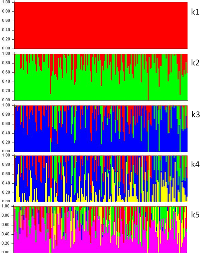
Each vertical line represents an individual and segment color represents the proportion of each group.
Figure 1 Structure and composition of El Uno Ranch American bison population based on five lines (k= 1, 2, 3, 4, 5).
In similar studies, the Bovine SNP50K chip was used in three bison populations (one European and two American), producing SNP percentages of 1.8, 2.6 and 2.9, and He estimates of 0.135, 0.197, and 0.19926,27. A SNP percentage in the same range (2.8 %) was reported for B. bonasus28, although higher values (9.35 %) have also been reported for European bison, with an accompanying Ho of 0.306 and He of 0.25029. Another study of European bison identified 1,536 SNPs, distributed at 8 to 136 SNPs per chromosome with an average of 51.230.
The current AB population in the United States of America is derived from a genetic bottleneck process with significant variability and genetic structure31,32. Three genetic lines were defined for the present study population. Given the origins of the El Uno Ranch herd, the line corresponding to the highest proportion probably corresponds to plains bison. A complementary line may be a contribution of the mountain bison and a third was likely generated by separation and development of the studied population. Any differentiation in the study population may have been caused by the genotype-environment interaction, although its adaptation and contribution to the ecosystem may also have had an effect. Genetic isolation between subpopulations affects some demographic and evolutionary processes; the consequent reduced gene flow can lead to accumulation of genetic differences between subpopulations33. Overall, differences within populations can derive from the genetic diversity of the founding ancestors and their relative contributions, as well as Ne and its evolution over time32. Genetic substructure does not always coincide with obvious morphological or geographic differences between subpopulations. Data from genetic markers and complementary analyses are required to draw contrasts between populations, identify possible sources of genetic material, and/or, where appropriate, define any possible differentiation. For example, a study of eleven bison populations identified genetic differentiation grouped into eight clusters32, while another study identified two genetically distinct subpopulations within the Yellowstone National Park herd33. Finally, an analysis of genetic structure in twelve bison herds identified three lines or genetic substructures (average constitution = 0.412, 0.303 and 0.285)34.
Conclusions and implications
Three genetic lines were identified within the El Uno Ranch American bison herd. Two may be associated with the source populations while a third is probably linked to the separation process and the effects of natural selection or genetic drift. The present results highlight the need to consider genetic variability and parentage levels when designing reproduction and conservation plans.
Literatura citada
1. Halbert ND, Terje R, Bhanu PC, James ND. Conservation genetic analysis of the Texas state bison herd. J Mammalogy 2004;85:924-931. [ Links ]
2. Freese CH, Aune KE, Boyd DP, Derr JN, Forrest SC, Gates CC, et al. Second chance for the plains bison. Biol Conser 2007;136:175-184. [ Links ]
3. Hedrick PW. Conservation genetics and North American bison (Bison bison). J Heredity 2009;100:411-420. [ Links ]
4. Gates CC, Curtis HF, Peter JPG, Mandy K. American Bison: Status survey and conservation guidelines. American Bison Specialist Group. 2010. [ Links ]
5. Anderson S. Mammals of Chihuahua: taxonomy and distribution. B Amer Mus Nat Hist 1972;148:149-410. [ Links ]
6. List R, Ceballos G, Curtin C, Gogan PJP, Pacheco J, Truett J. Historic distribution, and challenges to Bison recovery in the northern Chihuahuan desert. Conser Biol 2007;21:1487-1494. [ Links ]
7. List R, Pacheco J, Ponce E, Sierra-Corona R, Ceballos G. The Janos Biosphere Reserve. Northern Mexico. I J Wilderness 2010;16:35-41. [ Links ]
8. Solbrig OT. The origin and function of biodiversity. Environment: Sci Pol Sust Develop 1991;33:16-38. [ Links ]
9. Segura-Correa JC, Montes-Pérez RC. Razones y estrategias para la conservación de los recursos genéticos animales. Rev Biom 2001;12:196-206. [ Links ]
10. FAO. Management of small populations at risk: Secondary guidelines for development of National Farm Animal Genetic Resources Management Plans. 1998. [ Links ]
11. Toro MA, Caballero A. Characterization and conservation of genetic diversity in subdivided populations. Phil Trans Royal Soc B: Biol Sci 2005;360:1367-1378. [ Links ]
12. Toro MA, Fernández J, Caballero A. Molecular characterization of breeds and its use in conservation. Livest Sci 2009;120:174-195. [ Links ]
13. Lenstra JA, Groeneveld LF, Eding H, Kantanen J, Williams JL, Taberlet P, et al. Molecular tools and analytical approaches for the characterization of farm animal genetic diversity. Anim Genet 2012;43:483-502. [ Links ]
14. Waples RS. A bias correction for estimate of effective population size base on linkage disequilibrium at unlinked loci. Cons Genet 2006;7:167-184. [ Links ]
15. Goudet J. FSTAT: A computer program to calculate F-Statistics. J Heredity 1995;86:485-486. [ Links ]
16. Peakall R, Smouse PE. GenAlEx 6.5: genetic analysis in Excel. Population genetic software for teaching and research - an update. Bioinformatics 2012;28:2537-2539. [ Links ]
17. Waples RS, Do CHI. LDNE: a program for estimating effective population size from data on linkage disequilibrium. Mol Ecol 2008;8:753-756. [ Links ]
18. Kalinowski ST, Wagner AP, Taper ML. ML-Relate: a computer program for maximum likelihood estimation of relatedness and relationship. Mol Ecol Notes 2006;6:576-579. [ Links ]
19. Pritchard JK, Stephens M, Donnelly P. Inference of population structure using multilocus genotype data. Genetics 2000;155:945-959. [ Links ]
20. Evanno G, Regnaut S, Goudet J. Detecting the number of clusters of individuals using the software STRUCTURE: a simulation study. Mol Ecol 2005;14:2611-2620. [ Links ]
21. Earl DA, vonHoldt BM. Structure Harvester: a website and program for visualizing Structure output and implementing the Evanno method. Conserv Genet Res 2012;4:359-361. [ Links ]
22. Keller LF, Waller DM. Inbreeding effects in wild populations. Trends Ecol Evol 2002;17:230-241. [ Links ]
23. Skotarczak E, Szwaczkowski T, Ćwiertnia P. Effects of inbreeding, sex, and geographical region on survival in an American bison (Bison bison) population under a captive breeding program. Europ Zool J 2020;87:402-411. [ Links ]
24. Tokarska M, Kawałko A, Wojcik JM, Pertoldi C. Genetic variability in the European bison (Bison bonasus) population from Białowieża forest over 50 years. Biol J Linnean Soc 2009;97:801-809. [ Links ]
25. Pertoldi C, Bijlsma R, Loeschcke V. Conservation genetics in a globally changing environment: present problems, paradoxes and future challenges. Biod Conserv 2007;16:4147-4163. [ Links ]
26. Pertoldi C, Wojcik JM, Tokarska M, Kawalko A, Kristensen TN, Loeschke V, et al. Genome variability in European and American bison detected using the bovine SNP50 BeadChip. Conserv Genet 2010;11:627-634. [ Links ]
27. Pertoldi C, Tokarska M, Wojcik JM, Kawalko A, Randi E, Kristensen TN, et al. Phylogenetic relationships among the European and American bison and seven cattle breeds reconstructed using the Bovine SNP50 Illumina genotyping BeadChip. Acta Theriol 2010;55:97-108. [ Links ]
28. Kaminski S, Olech W, Olenski K, Nowak Z, Rusc A. Single nucleotide polymorphism between two lines of European bison (Bison bonasus) detected by the use of Illumina Bovine 50K BeadChip. Conserv Genet Res 2012;4:311-314. [ Links ]
29. Eugeniu MA, Adrian IO, Acatincai S, Neamt RI, Valentin CM, Ilie DE. Single nucleotide polymorphism in Bison identified by GGP Bovine 50K SNP assay. Anim Sci Biotech 2019;52:47-55. [ Links ]
30. Wojciechowska M, Nowak Z, Gurgul A, Olech W, Drobik W, Szmatola T. Panel of informative SNP markers for two genetic lines of European bison: Lowland and Lowland-Caucasian. Anim Biod Conserv 2017;40.1:17-25. [ Links ]
31. Boyd DP, Gates CC. A brief review of the status of plains bison in North America. J West 2006;45:15-21. [ Links ]
32. Halbert ND, Derr JN. Patterns of genetic variation in US federal bison herds. Mol Ecol 2008;17:4963-4977. [ Links ]
33. Halbert ND, Gogan PJP, Hedrick PW, Wahl JM, Derr JN. Genetic population substructure in bison at Yellowstone national park. J Heredity 2012;103:360-370. [ Links ]
34. Cronin MA, MacNeil MD, Vu N, Leesburg V, Blackburn HD, Derr JN. Genetic variation and differentiation of bison (Bison bison) subspecies and cattle (Bos taurus) breeds and subspecies. J Heredity 2013;104:500-509. [ Links ]
Received: May 29, 2022; Accepted: October 05, 2022
 Este es un artículo publicado en acceso abierto bajo una licencia Creative Commons
