


 text in
  English (pdf)
 Article in xml format
 Article references
 Send this article by e-mail
 Cited by SciELO
  Similars in
SciELO
Similars in
SciELO 
 Permalink
Introduction
Sheep farming for meat production in Brazil has expanded in the last decade because of the increased demand for this type of meat in the market. Thus, producers have sought ways to establish production systems capable of efficiently generating quality meat at a low cost1,2,3. However, the productivity of these animals in Brazil is still incipient due to deficiencies in genetic and nutritional management, poor financing, inadequate management systems of the various rearing stages, and low ability to properly organize the production chain4. Another relevant fact is that over 50 % of sheep production is carried out on natural pastures without management4. These peculiarities make the decision-making process in sheep production systems fraught with risks and uncertainties.
Despite being an inherent characteristic of animal production systems, the risk (likelihood of occurrence of an event) can be minimized through the adoption of tools that help decision-making5. In this sense, a lack of knowledge will result in the impossibility of estimating risk (uncertainty). Some information within and outside the production system is essential to reduce uncertainties associated with decision making6. Outside the production system, the producer has little control over the actions that impact the profitability of production. In contrast, actions within the farm will directly impact the success of the activity.
In this context, an adequate methodology for decision-making analysis requires accurate information about the problem as well as efficiency in handling the system, so the planned goals can be achieved7. Modelling is a tool that can aid the decision-making process, as it allows decision-makers to evaluate the behaviour of variables and their interrelationships, in addition to using previous or related information to predict results and simulate different scenarios8).
The use of mathematical models allows producers to estimate some important information that would be difficult to obtain in practical terms, e.g., herbage intake using correlated variables9. Modelling also makes it possible to monitor the weight of an animal and determine the best time for its sale10,11. In addition, it allows producers to estimate the weight of the carcass and major cuts before slaughter12,13. All this information is directly associated with the profitability and success of the production activity.
Thus, because of the different applications of mathematical models in production systems, this literature review examines concepts in modelling studies and the importance of using predictive models in the production of meat sheep.
Mathematical models
The use of mathematical models has become an indispensable tool for public policymakers and scientists14. Pool15 suggested that the act of modelling would become a third domain of science, joining the traditional domains of theory and experimentation. In this sense, important political decisions, such as the effect of global warming on terrestrial biology16,17, public health, and pandemic management18, have come to depend heavily on modelling studies. In addition, researchers have started to use modelling in the most diverse fields of science, e.g. medicine19, economics20, physics21, chemistry22, engineering23, law24, animal science25,26, and many others.
There are several concepts for mathematical models. Hamilton14 defined them as the expression of theory, which provides a possibility of comparing the theory with data obtained in the physical environment. For Tedeschi25, models are mathematical representations of mechanisms that govern natural phenomena that are not fully known, controlled, or understood. More recently, Tedeschi and Mendez8) postulated that mathematical models are arithmetic representations of the behaviour of real devices and life processes. All these authors also considered that models are an abstraction and a representation of reality8,14,25.
The use or non-use of mathematics defines whether the model is predictive or descriptive, respectively. Descriptive models theoretically address the performance of variables and their interrelationships. In contrast, predictive models are aimed at using prior information to predict results or simulate different scenarios8. In this respect, Tedeschi and Mendez8 categorized mathematical (predictive) models into three main classes: in a temporal context, models can be classified as static or dynamic; in a natural context, as empirical or mechanistic; and, in a behavioural context, as deterministic and stochastic.
Dynamic models are those that describe changes that have occurred and the obtained responses as a function of time. The non-linear models used to describe animal growth have a dynamic character27,28. Static models, on the other hand, are those that generate a response for a fixed instant, that is, they do not include time as a variable8. However, Tedeschi and Mendez8 warn that the concept of static versus dynamic depends on the time scale used, as a biological phenomenon can be better represented by a dynamic model when daily changes occur, but when years are used as a time variant, a static model may work better than a dynamic model, since daily changes are irrelevant to the variable of interest.
Empirical models are obtained from observational data. These models are applied in experimental studies that evaluate dose-response relationships, e.g., the effect of nitrogen rates on the crude protein content of forage plants. Thus, it is possible to estimate the concentration of a crude protein (variable Y) at any nitrogen rate (variable X) through polynomial regression fitting29. Mechanistic models, on the other hand, consider the underlying conceptual mechanisms and the combination of elements from different hierarchical levels. The main purpose of these models is to explain how an element at a higher level behaves or responds to a range of elements at a lower level. This type of model can be better exemplified in the modelling of the herbage accumulation dynamics of a given forage plant30. In this case, the mechanistic model seeks to explain the sequence of actions of abiotic factors at the level of molecules, cells, tissues, organs, tillers, plants, clumps, and the forage canopy.
Stochastic models are those that associate a risk or probability with the decision. Stochasticity is associated with a lack of understanding of the biological phenomenon. Accordingly, a greater understanding of the phenomenon would translate into a less stochastic model. An example of a stochastic model was developed by Nadal-Roig et al5 to address tactical decisions, plan production, increase flexibility, and improve the coordination and overall production of swine under the uncertainty associated with the price of animal sales. The authors concluded that the stochastic model was efficient in predicting the best scenario for the production system. Furthermore, due to the market uncertainty of the sales price for swine, the stochastic version led to more precise and realistic results than the deterministic version.
In contrast, deterministic models do not associate any probability with a given estimate8. Therefore, whenever the model is run without changes in the input variables, the same output information will be obtained. An example of the use of this type of model was proposed by the NRC31 to estimate dry matter intake by sheep. According to the NRC31, the dry matter intake (kg/day) of sheep is determined by the following input variables: adult body weight (kg), body weight, and standard reference weight, which would correspond to an adult animal. If female, it should be considered non-pregnant and non-lactating, with a body score of 2.5 on a scale of 1 to 5, and having already undergone complete skeletal growth. In this way, every time the model is run using the same input information, the predicted intake will be the same. However, the model does not give any probability that the predicted intake will indeed be observed.
Regardless of the type of model, its basic structure is composed of variables, parameters, and constants, but not all models exhibit these three components simultaneously. Variables-dependent or independent-are changed according to the individual; parameters vary depending on the model, and the constants do not vary in any situation. In this sense, two processes are commonly used for the creation of models: 1) Establishing ideas and concepts through an in-depth study of the literature and then creating parameters for the model variables, or 2) Analyzing experimental data that explain a biological phenomenon and then combining them into an equation25. In both situations, proper statistical analysis to assess the fit of the models is an indispensable step.
Evaluation of mathematical models
There are conceptual differences between the terms ‘validation’, ‘verification’, and ‘evaluation’ of mathematical models14,25. However, the term ‘model validation’ was frequently questioned by researchers25,32. Because models are considered an abstraction of reality and an approximation of the real system8,14,25, it is impossible to prove that all model components will truly predict the behaviour of a biological system. Tedeschi25 proposed the terms ‘evaluation’ or ‘test’ to indicate the degree of robustness of the model based on pre-established criteria. The author also highlighted that mathematical models cannot be proved valid, except if they are suitable for the purpose for which they are intended, under certain conditions.
In modelling studies, a protocol must be followed to define the best prediction model for the established goal. Thus, the process first requires an extensive review of the literature on the topic addressed. After a theoretical understanding of the phenomenon to be modelled is achieved, the next step is to adjust, evaluate, and compare the defined models and, finally, interpret the results and make inferences about the application of the selected models. Therefore, it is understood that evaluation is a fundamental step in the adjustment of prediction models25, as this step defines whether the model is suitable for its intended purpose. According to Hamilton14, model evaluation is a comparison of predicted over observed data, which uses statistical tools to support conclusions.
Accuracy and precision are two important concepts when evaluating mathematical models. Accuracy indicates the proximity of predicted to observed mean values. Precision, on the other hand, is the model's ability to consistently predict values25. Therefore, an accurate but not precise model (situation 1 in Figure 1) estimates an average value close to the true average value, but with a high standard deviation. In contrast, a model with low accuracy and high precision (situation 4 in Figure 1) predicts a mean different from the observed data but denotes a low standard deviation in the predictions. In situations 2 and 4 (Figure 1) the models are equally accurate, yet only model 2 shows the characteristics of accuracy and precision, as the points are distributed compactly in the center of the target.

The first and simplest assessment of the goodness-of-fit of models (precision and accuracy) is moment analysis of predicted and observed data. In this type of assessment, a good model is expected to estimate mean, maximum, and minimum values as well as data variance and standard deviation close to the observed values33. Spearman's correlation coefficient value has also been used initially to assess the classification of predicted and observed data values. This coefficient assesses whether the highest predicted value is also the highest observed value, thus creating a classification among all data34.
Linear regression between observed and predicted values is commonly used to evaluate models. The hypothesis that the predicted data are equal to the observed data is tested by the regression equation Y = β0 + β1 × X, where Y is the observed value; β0 and β1 represent the intercept and slope of the regression equation, respectively; and X is the value predicted by the equations. Model-predicted values are plotted on the X-axis, whereas observed values are plotted on the Y-axis25. In this graph format, the data points located above and below the equality line indicate overestimation or underestimation by the model, respectively26.
To test the hypothesis (β0 = 0 and β1 = 1), Dent and Blackie35 suggested simultaneously evaluating whether the intercept is different from zero and the slope is different from one. For this purpose, the simultaneous F test for the identity of the regression parameters predicted by observed data was used36. However, Tedeschi25 warned that the F test is valid only for deterministic models and should not be used for stochastic models. In addition, due to the assumption that the data are independent, which is not always observed in a modelling study, the simultaneous F test can result in errors of acceptance or rejection of the tested hypothesis36.
After obtaining the linear regression, it is possible to calculate the coefficient of determination of the equation (R 2 ). The coefficient of determination indicates the percentage of variation in Y that is explained by X. Therefore, R 2 evaluates the proximity of the data to the fitted regression line. It is noteworthy that the interpretation of the R 2 value is often wrong33. When used in isolation, this information is not a good indicator of the quality of the model, as R 2 measures the precision and not the accuracy of the equation. Coupled with this is the fact that a high coefficient of determination does not necessarily imply that there is a linear relationship between predicted and observed data since the relationship can be curvilinear25.
Another way to evaluate the regression equation is by the mean square error (MSE), which evaluates the precision of the adjusted linear regression using the difference between the observed values and the values estimated by the regression. Analla37 recommended MSE as the best criterion to select the model with the best fit when comparing several models. It should be noted that although several methods are used to assess the adequacy of the regression equation, its use may generate ambiguous results when data do not show the normal distribution and in cases in which residual errors are low25. In this context, some additional evaluations are carried out.
The MSE is similar to the mean squared error of prediction (MSEP). The fundamental difference between the two parameters is that MSEP is the difference between the observed values and the values predicted by the model, while MSE, as seen above, is the difference between the observed values and the values estimated by the regression. Tedeschi25 considered MSEP the most common and reliable measure to determine the predictive accuracy of a model; however, the author warned that its reliability will decrease as the number of observations decreases. In addition, the author highlighted that MSEP does not provide any information about the precision of the model and that a disadvantage of MSEP is that deviations are weighted by their squared values, which removes the negative data, thus giving greater emphasis to larger values.
Bunke and Droge38 proposed a decomposition of MSEP that takes into account the source of variation of the parameters. By this fractionation, MSEP is divided into mean error, systematic error, and random error. When most errors are attributed to the mean error, it means that there is a deficiency in the placement of the equality line, which can be corrected with an additive correction factor. Systematic error, on the other hand, indicates a fault in line displacement, which can be corrected with a multiplicative correction.
The model's coefficient of determination (CD), which shows the proportion of the total variance of observed values that is explained by the predicted data, has long been used to evaluate mathematical models. However, the CD has been replaced by the concordance correlation coefficient (CCC) in studies of continuous variables39,40. The CCC simultaneously assesses the accuracy and precision of equations, which makes it a powerful measure. The CCC value is obtained by an equation of two components: 1) Correlation coefficient, which measures precision; and 2) Bias correction factor, which indicates accuracy41.
Numerous statistical techniques are used to assess the precision and accuracy of models. However, no technique used in isolation is capable of adequately evaluating model performance25. Therefore, the best way to assess the predictive performance of a model is to associate it with a set of statistical methods. It is important to emphasize that this review addresses the main methods used in modelling studies predicting the dry matter intake and carcass traits of sheep39,40,42. A further discussion on the evaluation of models from a statistical point of view was presented by Neter et al33 and Tedeschi25.
Application of predictive models in meat sheep production
Due to the diverse applications of mathematical models in sheep production systems, this literature review will address the application of modelling studies in predicting dry matter intake by grazing sheep as well as the body weight and carcass traits of sheep through biometric measurements. This information is difficult to obtain under practical conditions; however, it is directly associated with the profitability and success of the production activity. It is highlighted that the possibilities of using modelling in sheep production are as diverse as possible and it would be difficult to summarize all this information in a single review.
Prediction of dry matter intake by grazing sheep
In the case of feedlot animals, the chemical and physical characteristics of ingredients that make up the diets and their interactions have a great effect on dry matter intake (DMI)43,44. In short, the animal's energy demand defines the consumption of diets with high caloric density45. On the other hand, when the animal is fed diets of low nutritional value and low energy density, the physical capacity of the gastrointestinal tract determines the potential for DMI46. In this respect, Mcdowell47 mentioned that herbage intake is primarily influenced by body size since the size of the animal, is positively correlated with the nutritional requirements of maintenance42,43,45, followed by energy density and the rate of digestion of the diet. Furthermore, the author observed that DMI is positively correlated with organic matter digestibility.
The neutral detergent fibre (NDF) content of a diet or herbage is an efficient parameter to express the action of these two mechanisms to control dry matter intake, as it is positively related to the rumen-fill effect and inversely related to the energy concentration of the diet48.
Animal-related factors such as breed, sex, age, body weight, physiological stage (growth, pregnancy, or lactation), and body composition influence the nutrient requirements and intake of sheep45. Mertens48 suggested that nutrient intake depends on important factors related to feeding management (feed availability, linear trough area, feed accessibility, frequency of supply, physical form, and processing), in addition to environmental conditions and animal welfare related to the energy concentration of the diet48.
Regarding grazing animals, in addition to all the aforementioned factors acting on dry matter intake, the complex interactions between animal and pasture characteristics affect the nutrient intake rate49. Feeding behaviour is known to be the most efficient way to demonstrate the interactions between pasture structure and herbage intake50.
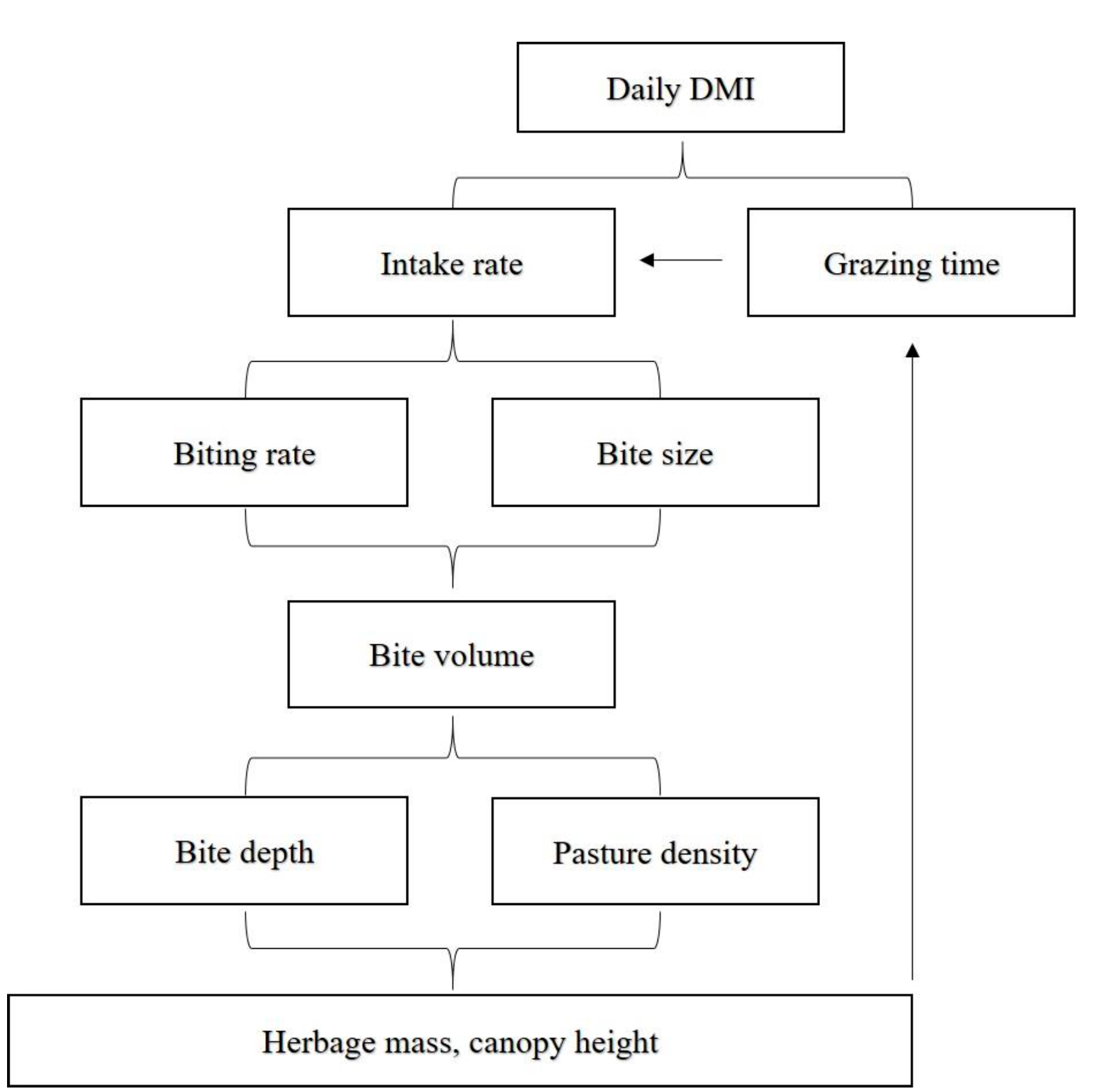
According to a mechanistic view, the daily DMI for grazing sheep is the result of the time spent by the animal in searching and prehending the herbage and the intake rate during this period50, which, in turn, is the product of biting rate and bite weight. The rate and weight of a bite change when the amount of herbage per bite (bite volume) is changed. The bite volume is sensitive to oscillations in bite depth and herbage bulk density, which in turn is determined by canopy height and herbage mass (Figure 2). The pasture structure (herbage mass, height, etc.) also changes the time spent by the animal on the grazing activity51,52.
To exemplify the relationship between pasture structure, feeding behaviour, and intake, one must simply imagine a situation with limitations on the herbage supply. In this circumstance, there is a reduction in bite-size, whereas grazing time and biting rate increase52. Therefore, to some extent, it is possible to obtain constant herbage intake in pastures with different canopies. Nonetheless, if the herbage allowance is too low, the increase in grazing time will not be able to maintain intake due to the reduction in intake rate54.
Thus, because of the existence of several factors influencing the DMI of grazing sheep, the modelling of this parameter becomes very complex. For this reason, most sheep DMI prediction models are obtained from experiments conducted in feedlot conditions31,42,43,45. This may lead to inconsistencies if they are used to predict the DMI of grazing sheep, as they do not consider the characteristics of the pasture and the interactions between the animal and the forage plant.
Most models used to predict intake by grazing animals are mechanistic, focusing on the digestive process and the selectivity of ingestion under grazing conditions, and they mainly consider pasture height or the amount of herbage removed50,55. Pittroff and Kothmann56 undertook a comparative analysis of quantitative models predicting the feed intake of sheep and observed that about 55 % of the equations took into account some pasture trait, with a predominance of herbage availability. The researchers concluded that there is a weak conceptual framework in the development of the models.
Of the models presented in the review by Pittroff and Kothmann56, that developed by Freer et al57 focused more on pasture characteristics. The equation predicts intake by sheep as the product of potential feed intake (Imax) and the proportion of that potential (relative intake) that the animal can obtain from the available amount of feed. Imax was defined as the amount ingested (kg/d of DM) when the animals are allowed unrestricted access to feed with a DM digestibility of at least 80 %, which depends on the standard weight of an adult animal (standard reference weight) and the ratio between body weight and standard reference weight (Equation 1). It is noteworthy that in the case of tropical grasses, the minimum digestibility of 80 % is hardly reached58,59,60.
Where SRW= standard reference weight; Z= relative animal size, the ratio of body weight to standard reference weight.
Relative intake was described as the product of two feed attributes: relative availability and relative ingestibility. For grazing animals, relative availability is mainly predicted from the herbage mass, whereas relative ingestibility is predicted from the digestibility of the pasture collected by grazing simulation (hand plucking)57.
To simulate the ruminant intake dynamics during grazing, Baumont et al50 developed a theoretical model of an intake rate that combines the pasture structure and the animal's decision to graze or perform other activities. The authors defined dry matter intake as the sum of instantaneous intake rates, which, in turn, are determined as a function of potential intake rates in grazing horizons, preferences that determine the proportions selected in both pasture horizons, and animal satiety levels (Equation 2).
Where IR= intake rate (g DM/min); PREFi and PREFi + 1= relative preference determined from a grazing decision sub-model that defines how the animal distributes intake between the highest available horizon (i) and the next available horizon (i + 1), according to the relative preferences PREFi and PREFi+1; SL= satiety level; PIRi= potential intake rate (g DM/min) obtained from the time taken by the animal to perform the bite and the weight of that bite in the highest available horizon (i), and the next available horizon.
McCall61 proposed a model to estimate herbage intake in pastures where perennial ryegrass is the predominant forage species. The author modelled the actual DMI of sheep on pasture as a function of the maximum intake multiplied by the correction factor (Equation 3). The correction factor is obtained from herbage allowance and the animal's potential intake (equations 4 and 5). Herbage allowance was estimated by harvesting the forage contained within 1-m2 metal frames.
Where HI= herbage intake (kg/day); Imax= maximum herbage intake (kg/day); M= correction factor; EXP= exponential (2.7182); HAM= herbage allowance divided by maximum intake; and HM= herbage mass minus dead material (kg/ha).
Medeiros62 used the model proposed by McCall61 to estimate the intake of sheep on Cynodon spp. under different grazing intensities in a continuous grazing system and concluded that the McCall61 model overestimated the animals’ intake. This overestimation indicated by Medeiros could be due to the type of grass since McCall worked with a C3 grass that is more digestible than the C4 with which Medeiros worked. Thus, Medeiros62 suggested replacing the green herbage allowance (leaf + stem) in the equation with a green leaf allowance. Only then was the estimated intake statistically equal to that observed.
Similarly, Gurgel et al9 evaluated different models predicting DMI in tropical pastures using the adjustment factor proposed by McCall61 and concluded that the equations do not accurately predict the DMI of meat sheep and generate overestimated values in tropical climate pastures. The authors proposed that the DMI estimate for lambs on tropical pasture should consider the following model (Equation 6):
Where DMI= dry matter intake (% LW); LW= live weight (kg); GT= grazing time (min/day); and GHA= green herbage allowance (kg DM/100 kg LW), which corresponds to herbage allowance minus dead material.
Therefore, the models proposed for a temperate climate do not correctly estimate herbage intake by sheep on tropical pasture. In this way, studies to estimate intake by sheep in tropical regions are necessary, especially in systems that adopt pasture as the primary source of nutrients, as this information is of fundamental importance for nutritional planning.
Prediction of body weight and carcass traits of sheep through biometric measurements
Body weight is one of the main pieces of information that guides decision-making in production systems due to its direct relationship with the nutritional requirements of animals31. In addition, monitoring the growth curve of ruminants makes it possible to identify the phases in which the animal is more capable of converting the consumed feed into body tissue and the best time for its sale10,11,63.
Animal growth is evaluated using direct measuring equipment, such as livestock scales. However, due to the conditions in which traditional sheep production systems operate4, the direct determination of the animals’ body weight often represents a challenge for producers because of the high cost of acquiring and maintaining scales64,65,66,67. In most cases, this causes producers to market animals based on visual scores, which leads to errors in the estimation of body weight and affects the profitability of production systems68.
The estimation of body weight by indirect methods can be an easily adopted, low-cost alternative. In this sense, biometric measurements are a viable option to predict body weight due to the correlation between these traits and the body weight of animals65,69. This method consists of developing mathematical models that allow producers to estimate bodyweight using some biometric measurements (Figure 3) from linear and multiple regression analyses. These body measurements can be obtained with a horse measuring stick and a measuring tape12,41, easy-to-handle and inexpensive instruments that do not require sophisticated periodic maintenance.
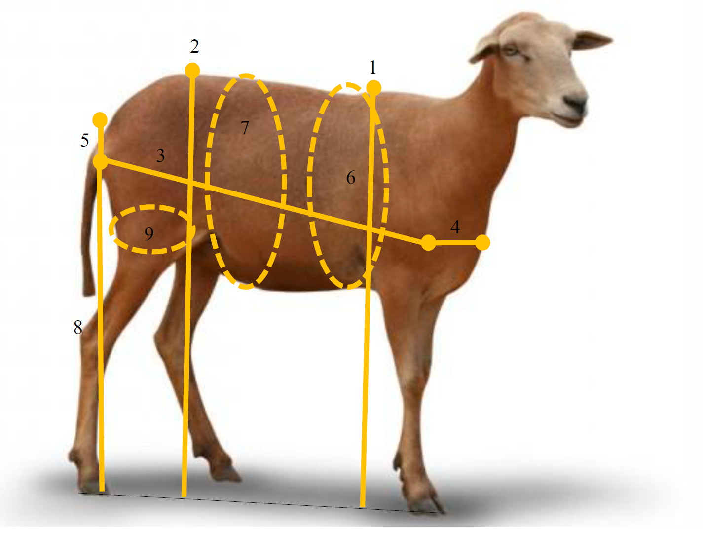
Withers height (1); rump height (2); body length (3); chest width (4); rump width (5); heart girth (6); abdominal circumference (7); leg length (8); leg circumference (9).
Figure 3 Main biometric measurements performed on sheep
The main biometric measurements (Figure 3) evaluated in sheep are as follows70: withers height (WH) - from the highest point of the withers to the ground (1); rump height (RH) - the vertical distance from the highest point of the rump to the ground (2); body length (BL) - from the scapulohumeral joint to the caudal part of the ischium (3); chest width (CW) - the measurement between the tips of the scapulae (4); rump width (RW) - the distance between the ischial tuberosities (5); heart girth (HG) - taken around the chest cavity (6); abdominal circumference (AC) - taken around the abdominal cavity (7); leg length (LL) - taken from the ischial tuberosity to the ground (8); and leg circumference (LC) - taken around the middle portion of the thigh (9).
Some studies were conducted to develop linear and multiple equations to estimate the bodyweight of sheep from biometric measurements65,66,71,72,73. The authors concluded that HG is the most important biometric measurement for predicting animal body weight (Table 1). In contrast, Canul-Solís et al66 used RW to estimate the body weight of Pelibuey sheep. However, when more than one measurement is used, the predictive capacity of the equations increases68,69,73,74.
Table 1 Equations to predict the body weight (BW) of sheep using biometric measurements (cm)
| Author | Breed | Equation | R2 |
|---|---|---|---|
| Chay-Canul et al65 | Pelibuey | BW (kg) = -47.97 + 1.07 × HG | 0.86 |
| Canul-Solís et al66 | Pelibuey | BW (kg) = - 19.17 + 3.46 × RW | 0.96 |
| Málková et al68 | Charolais; Kent; crossbred | BW = (kg) = -3.997 + 0.225 × HG | 0.78 |
| Málková et al68 | Charolais; Kent; crossbred | BW (kg) = -4.672 + 0.243 × CBC + 0.198 × HG | 0.80 |
| Gurgel et al69 | Santa Inês | BW (kg) = 0.45 × HG - 0.58× AC + 0.005 × AC2 + 0.002 ×RH2 | 0.88 |
| Kumar et al71 | Harnali | BW (kg) = -63.72 + 1.23 × HG | 0.87 |
| Worku73 | Kebeles; Arsi-Bale | BW (kg) = -39.51 + 0.91× HG | 0.71 |
| Worku73 | Kebeles; Arsi-Bale | BW (kg) = 45.77 + 0.59 × HG + 1.99 × CBC + 0.30 × CD + 0.5 × RH | 0.81 |
| Grandis et al74 | Texel | BW = (kg) -107.16 + 1.40 × HG + 0.60 × WH | 0.88 |
HG= heart girth, RW= rump width; CBC= cannon bone circumference; AC= abdominal circumference; RH= rump height; CD= chest depth; WH= withers height.
Another way to use biometric measurements to predict the body weight of sheep is from body volume, which is obtained by the formula used for calculating the volume of a cylinder, including the HG and BL measurements75:
Radius (cm)= HG / 2π,
Body volume (dm3)= (π × r2 × BL) / 1000,
where, r= radius of the circumference (cm); π= 3.1416; HG= heart girth (cm); and BL= body length (cm).
Salazar-Cuytun et al67 compared three equations (linear, quadratic, and exponential) to assess the relationship between body volume and weight in Pelibuey lambs and ewes. The authors observed a correlation coefficient of 0.89 between body volume and weight. Additionally, the quadratic model was found to have the best performance, according to the adequacy assessment. Le Cozler et al76 reported that body volume is strongly correlated with weight in lactating Holstein cows.
In addition to being an efficient method to estimate body weight, biometric measurements are used to predict sheep carcass traits12,40,77. Determining the yield of carcass or major cuts before slaughter is valuable information for production systems, as it allows the producer to estimate the gross income of the farm. In this regard, the use of biometric measurements taken before slaughter is of greater interest in commercial production conditions due to the low additional cost for producers40,78,79.
Because it is directly related to producer remuneration, the carcass weight has been the variable most predicted by biometric measurements, with slaughter weight explaining 47.0 to 99.0 % of the variation in ruminant carcass weight79,80. However, when biometric measurements are used in association with body weight in linear and multiple equations to predict carcass weight, there is an increase in the coefficient of determination40. In this respect, Gurgel et al81 showed that the measurements of CW, LC, and RW, together with body weight, explained 91.0 % of the variation in the carcass weight of Santa Inês lambs finished on tropical pasture. For Pelibuey lambs, Bautista-Díaz et al78 recommended an equation to estimate the carcass weight that is associated with the measurements of BL, HG, and AC and abdominal width (R2= 0.89). In predicting the hot carcass weight of Morada Nova lambs, Costa et al12 recommended an equation without using body weight as an independent variable. According to the authors, the measurements of BL, WH, CW, AC, and body condition scores are the most important in predicting the carcass weight of the studied sheep (R2= 0.80).
Sheep meat is sold mostly in the form of half carcasses or whole carcasses. Nevertheless, one way to add value to the meat is by selling it through cuts obtained by sectioning the carcass82. Thus, the carcass is initially divided into the major cuts of shoulder, neck, loin, leg, and rib, which are smaller and facilitate marketing, conservation at home, and preparation for consumption3,82,83.
Biometric measurements are highly correlated with the major cuts of the carcass2. Therefore, studies were developed to test the hypothesis that biometric measurements would be efficient in predicting the yield of these cuts. Shehata13 developed regression models to predict the weight of the major cuts of the carcass of Barki lambs from biometric measurements and found that HG explained 67.0 % of the variation in leg weight, and when HG was associated with BL, this value rose to 72.0 %. In addition, Shehata13 observed that the HG and BL precisely estimate the weights of the loin roast, shoulder, and loin chop cuts. Abdel-Moneim84 indicated BL as an efficient variable to predict the shoulder weight of Barki sheep.
The application of biometric measurements is not restricted to predicting carcass weight and major cuts. When used in equations, these measurements estimate the amount of internal fat and carcass trimmings, ribeye area, and the yield of non-carcass components, muscles, bones, and adipose tissue12,40,77. Thus, the monitoring of biometric measurements is a management tool that can help production systems increase revenues and shorten the time needed for animals to reach slaughter weight.
It is noteworthy that, for the most part, these measurements are carried out on feedlot-finished animals and/or in wool sheep, which does not represent the reality of production systems in tropical regions, since tropical forage grasses are the food base of small and large ruminants and are responsible for most of the meat produced in the tropics. Therefore, modelling studies must be developed to estimate the weight and carcass traits of hair sheep finished in tropical pastures through biometric measurements, taking into account that genotype, sex, age, rearing system, and health can change carcass traits and composition85,86.
Conclusions and implications
Despite its low adoption rate, modelling has great potential to help in decision-making in meat sheep production. Modelling is a tool capable of predicting the dry matter intake, bodyweight, carcass weight, and major marketable cuts of sheep with high precision and accuracy, through correlated measurements. These equations can be used by researchers, producers, technicians, and the meat industry, thus facilitating activity planning. However, further research is warranted to increase the databases so that the equations can be applied in the most diverse scenarios. In addition, more studies are needed to predict herbage intake using information more easily obtained in practical production conditions.

