


Serviços Personalizados
Journal
Artigo
 texto em
  Inglês (pdf)
 Artigo em XML
 Referências do artigo
 Enviar este artigo por email
Indicadores
-
 Citado por SciELO
 -
 Acessos
Links relacionados
-
 Similares em
SciELO
Similares em
SciELO
Compartilhar

 Permalink
Revista mexicana de ciencias pecuarias
versão On-line ISSN 2448-6698versão impressa ISSN 2007-1124
Rev. mex. de cienc. pecuarias vol.14 no.1 Mérida Jan./Mar. 2023 Epub 24-Mar-2023
https://doi.org/10.22319/rmcp.v14i1.6162
Articles
Estimation of forage mass in a mixed pasture by machine learning, pasture management and satellite meteorological data
a Universidad Autónoma de Querétaro. Facultad de Ciencias Naturales. 76230 Juriquilla, Santiago de Querétaro, Querétaro, México.
b Universidad Nacional Autónoma de México. Facultad de Medicina Veterinaria y Zootecnia, Centro de Enseñanza, Investigación y Extensión en Producción Animal en Altiplano CEIEPAA. Querétaro, México.
c Universidad Autónoma Chapingo. Departamento de Zootecnia, Posgrado en Producción Animal. Estado de México, México.
Measuring forage mass (FM) in the pasture, prior to grazing, is critical to determining the daily allocation of forage in pastoral animal production systems. FM is estimated by cutting forage in known areas, using allometric equations, or with the use of remote sensors (RS); however, the accuracy and practicality of the different methods for estimating FM is variable. The objective was to obtain predictive models using environmental and pasture management variables to predict FM. Regression models were fitted to estimate FM based on variables of pasture management (PM) or measurements obtained by RS, such as reflectance, air temperature, and rainfall. A mixed pasture grazed by beef cattle was studied for three years. With 80 % of data, models were built by ordinary least squares (OLS) or by machine learning (ML) algorithms. The remaining 20 % of the data was used to validate the models using the coefficient of determination and average bias between estimated and observed values. The base model of study was the relationship between pasture height before grazing and FM, this model was fitted using OLS; the r2 was 0.43. When models that included PM variables were fitted, the r2 was 0.45 for OLS and 0.63 for ML. When fitting models with PM and RS variables, the r2 was 0.71 for OLS and 0.96 for ML. ML-fitted model ensembles reduced the bias of FM estimates of the examined pasture. Overall, ML models better represented the relationship between pasture height before grazing and FM than OLS models, when fitted with pasture management variables and RS information. ML models can be used as a tool for daily decision-making in pastoral production systems.
Key words Alfalfa; Forage; Rain; Lucerne; Temperature; Remote sensors
Medir la masa de forraje (MF) en la pradera, antes del pastoreo, es fundamental para determinar la asignación diaria de forraje en sistemas pastoriles de producción animal. La MF se estima por corte de forraje en áreas conocidas, utilizando ecuaciones alométricas, o con el uso de sensores de percepción remota (PR); sin embargo, la exactitud y practicidad de los distintos métodos para estimar la MF, es variable. El objetivo fue obtener modelos predictivos usando variables ambientales y del manejo de la pradera para predecir la MF. Se ajustaron modelos de regresión para estimar la MF con base en variables del manejo de la pradera (MP) o mediciones obtenidas por PR, como reflectancia, temperatura del aire y lluvia. Por tres años se estudió una pradera mixta pastoreada con bovinos productores de carne. Con 80 % de datos se modeló por mínimos cuadrados ordinarios (OLS) o por algoritmos de aprendizaje automatizado (ML). El 20 % restante de los datos se utilizó para validar los modelos usando el coeficiente de determinación y el sesgo promedio entre valores estimados y observados. El modelo base de estudio fue la relación entre la altura de la pradera antes del pastoreo y la MF de este modelo se ajustó usando OLS; la r2 fue 0.43. Cuando se ajustaron modelos que incluyeron variables del MP, la r2 fue 0.45 para OLS y 0.63 para ML. Al ajustar modelos con variables de MP y PR, la r2 fue 0.71 para OLS y 0.96 para ML. Los ensambles de modelos ajustados con ML redujeron el sesgo de estimados de MF de la pradera examinada. En general, los modelos de ML representaron mejor la relación entre altura de la pradera antes del pastoreo y MF que los de modelos de OLS, al ajustarlos con variables de manejo de la pradera y con información de PR. Los modelos de ML pueden usarse como herramienta para la toma de decisiones diaria en sistemas productivos pastoriles.
Palabras clave: Alfalfa; Forraje; Lluvia; Temperatura; Sensores remotos
Introduction
Animal production using grazed pastures depends on the rate of accumulation of forage mass (FM), as well as on the timely allocation of an adequate stocking rate to take advantage of the FM; other important aspects are nutritional quality and seasonality in the rate of accumulation of FM. Cost-effective management of a pasture through direct grazing involves, among other things, implementing grazing management without compromising vegetation cover regrowth, as well as accurately knowing the FM in the pasture before and after grazing1. Traditionally, FM is measured directly with forage cuts in quadrants of known area, distributed in a spatially representative manner and in a sufficient number that represents the variability of the vegetation cover in the pasture2,3. The cutting of quadrants is laborious and therefore methods and devices have been developed for the indirect estimation of FM4-6. Pasture canopy height, measured with a sward stick, is useful to represent the FM, although the relationship may be different depending on the botanical composition, density of the pasture canopy and season of the year7-9. The height of the compressed forage measured with a rising plate meter estimates the FM considering the density of the canopy and is a very common practice at the farm level in countries such as New Zealand2. The relationship between canopy height and FM in ryegrass and white clover pastures is well known and routinely applied in New Zealand10; for pastures with other forage species such as alfalfa, more research is needed to determine the relationship between canopy height and FM8.
Remote sensing (RS) by orbital satellites measures spectral reflectance, the proportion of incident energy reflected by the Earth’s surface at different wavelengths; these measurements have been associated with vegetation activity processes11. With RS information, it is also possible to estimate environmental variables such as temperature, rainfall, and others12. The wide availability and free access of RS products is an opportunity to explore crop dynamics and establish relationships with productive parameters, such as FM. The time series available for different RS products allow retrospective studies to be made, which is valuable for evaluating pasture management practices and regional grassland studies. However, the spatial scale of measurement is coarse in some RS sensors and is an important disadvantage in studies such as the one described in this research.
Recently, a variety of machine learning (ML) algorithms have been incorporated into regression analysis and they are an alternative to ordinary least squares (OLS) regression. Photosynthesis in ecosystems, named gross primary productivity and net primary productivity (when discounting losses by respiration), has been modeled with empirical or mechanistic approaches, from OLS models to those that simulate ecophysiological processes at the global level based on RS13. Net primary productivity includes photosynthetic partitioning into aerial and root biomass and therefore does not reflect the FM available for grazing. Lang et al14 estimated arid grassland production using measurements from rainfall RS sensors, spectral reflectance obtained from the Landsat 7 satellite and random forest; a ML algorithm. Using Neural Networks, another ML-type algorithm, Chen et al15 related the spectral reflectance measured by the Sentinel-2 satellite and FM on dairy farms of Tasmania in Australia. In these studies, the coefficient of determination (r2) in different models was between 0.6 and 0.7. Conceptually, it is important to incorporate humidity conditions, in the short or medium term, to explain the carrying capacity of the grassland16, since water is the main limiting resource of plants in arid and semi-arid environments. The conditions of water availability for plants can be represented by the precipitation (P) that occurred, water available in the soil or vapor deficit in the atmosphere. However, to explain the FM, not only the P occurred in the period of accumulation of the FM (month in which the FM was measured) is important, but also the humidity conditions that occurred in previous months.
In the present work, the relationship between FM and pasture height was examined as a baseline to compare other models that used meteorological variables obtained by RS or in conjunction with variables representative of pasture management (PM) conditions; such as the grazing and rest periods of the grazed area or the pasture height itself. In particular, the usefulness of models to predict FM based on previous rainfall and temperature conditions in different time windows was explored; for example, the P accumulated in the previous month, in two months or three months before the measurement of the FM. The objective was to obtain a predictive model of FM that could be incorporated into grazing planning. For this purpose, three years of measurements on a mixed of alfalfa-grass pasture grazed by beef cattle, were used.
Material and methods
Site
The study was carried out at the Centro de Enseñanza, Investigación y Extensión en Producción Animal en el Altiplano, run by Facultad de Medicina Veterinaria y Zootecnia from the Universidad Nacional Autónoma de México. The site is located at 20° 36’ 13.88” N, 99° 55’ 02.91” W and altitude of 1,913 m asl. The climate is extreme dry Ganges type without dry spells, BS1 0w(e)g, according to the historical climatological records (1951 to 2006) of climatological station 22025; the closest to the site, where the annual averages of precipitation and temperature are 458 mm and 23.5 °C17.
The pasture was established in 2004 with a mixture of 50 % alfalfa (Medicago sativa) and grasses such as orchard grass (Dactylis glomerata), tall fescue (Festuca arundinaceae) and perennial ryegrass (Lolium perenne). The grazing area was 19 ha divided into 16 paddocks of equal size and delimited through mobile electric fence. The pasture was irrigated with a center-pivot sprinkler system; however, there were no records of the irrigation sheet or calendar. The grazing mob was made up of 88 dams of the Limousin breed and their calves. The grazing time in each division was established based on: the estimation of FM, proximate chemical analysis of FM samples, and the dry matter (DM) allowance for the mob in each turn. Reproductive management was mainly with artificial insemination and year round calving.
Data
From 2008 to 2010, 399 FM observations were obtained prior to grazing of the allocated grazing area. Each FM observation corresponded to the beginning of a grazing cycle of the mob. The observations were considered experimental units, and each consisted of eight random measurements obtained with the modified quadrat technique; to protect the alfalfa regrowth the pasture samples were cut to 10 cm height in an area of 0.25 m218. Forage samples were dehydrated in a forced-air oven for 48 h to determine the DM content and the data was expressed in kg DM ha-1. In each grazing cycle, the following were recorded: the height of the pasture (H_pasture), the date of grazing (Day_grazing and Month_grazing), grazing time (G_time), resting time of the grazed area from the previous grazing (R_time), month of the beginning of growth in the previous grazing cycle (Month_beg_grow) and the average monthly pasture accumulation rate of DM (PAR, kg DM ha-1 d-1). These variables were collectively referred to as pasture management (PM) variables.
Using the Application for Extracting and Exploring Analysis Ready Samples of the Land Processes Distributed Active Archive Center of the National Aeronautics and Space Administration (NASA), the MCD43A4 version 619 product was requested. The MCD43A4 product is generated from measurements made by Moderate-Resolution Imaging Spectroradiometer (MODIS) sensors at a spatial resolution of 500 m2. This product consists of seven reflectance bands adjusted by the Bidirectional Reflectance Distribution Function and produced daily, which are a moving average of the contiguous 16 days measurements. Data from eight contiguous pixels corresponding to the polygon of coordinates: 99.93 W, 20.60 N to 99.92 W, 20.61 N, were downloaded. The radiation spectrum (nm) covered by bands one to seven is (b1-b7): 620-670, 841-876, 459-479, 545-565, 1230-1250, 1628-1652 and 2105-2155. Rainfall data were from the 3IMERG version 6 product of the Global Precipitation Measurement Mission of NASA obtained through the Giovanni portal (https://giovanni.gsfc.nasa.gov/giovanni). The P data (mm) was the monthly accumulated for the coordinate 99.92 W, 20.60 N; the spatial resolution of 3IMERG is 10 km2. Through the Giovanni portal, the MODIS MOD11A2 version 6 product of daily surface temperature during the day (LST_d) and night (LST_n) was also obtained.
For MODIS, good quality was determined according to the quality data accompanying the respective products. In the R20 language, a code was generated to find the measurement dates of the MCD43A4 closest to the measurement date of the FM. Using Qgis v3.16.421 and a satellite image from Google Maps22 as a guiding template, a vector layer corresponding to the area of irrigation by central pivot was determined; the circle comprised different area of the sampled pixels of the MCD43A4. For each reflectance band, the average corresponding to the vector was obtained using the extract function of the raster package.
Variable generation
The reflectance in the bands b2 and b1 is associated with the ability of vegetation to absorb photosynthetically active light and there are different indices to represent this activity of the vegetation. The normalized vegetation index (NDVI) and the enhanced vegetation index (EVI) were calculated using the spectral bands of the MCD43A4 product:
With the time series of P, the following variables were calculated: the P accumulated in the previous month (P_lag_1), the P accumulated in the previous two months (P_lag_2) and so on until the P accumulated in six previous months: (P_lag_3, P_lag_4, P_lag_5 and P_lag_6). For LST_d and LST_n, the average of the previous month (LST_x_avg_1), of the previous two months (LST_x_avg_2) or of the previous three months (LST_x_avg_3), where x represents the indicative d or n, for day or night, was calculated. These variables represented the prevailing environment before measuring FM.
Modeling
The baseline model for comparison was the linear regression between FM and H_pasture. Four modeling scenarios according to the type of algorithm were explored: ML or OLS and the type of variables available for modeling: using only explanatory variables of RS origin (ML_RS and OLS_RS) or RS variables and those of PM (ML_RS_PM and OLS_RS_PM). The models were trained with 80 % of observations chosen randomly and 20 % were reserved for evaluation. Model evaluation is a black box concept about the relevance of the result of the model23. The statistical procedures were carried out in the R language, the name of the packages is indicated where relevant. An orthogonal regression (major axis regression) model was fitted between observed values and predicted values using the smatr 3 package, since observed FM values are measured with error24. The following were calculated: coefficient of determination (r2), root mean square error (RMSE), the Akaike (AIC) and Bayesian (BIC) information criteria, deviance, and bias. These quantitative indicators, as well as graphical evaluation, are techniques commonly used to evaluate mathematical models for predictive purposes25.
In the case of OLS, the variance inflation value (VIF) was used to identify multicollinearity using the stepAIC and vif26 functions; 10.0 was the maximum allowed value of VIF to retain variables in the OLS multiple regression model. The significance level was set at 0.05 for parametric analyses and residual analysis of the OLS regression.
The ML model was generated with the h2o.automl function of the H2O27 package, it produces a set of models with different algorithm realizations: deep learning (DL), feedforward artificial neural network (NN), general linear models (GLMs), gradient-boosting machine (GBM), extreme gradient-boosting (XGBoost), default distributed random forest (DRF) and extremely randomized trees (XRT). Each individual model can be used to predict the response, but also to generate two types of model ensemble: one is from all the algorithms used in the generated models, and the second type of ensemble only considers the best models of each class or family of algorithms; both types of ensembles generally produce better predictions than individual models23.
The h2o.automl function was run twenty times with the following parameters: a) max_runtime_secs = 500, the maximum runtime before training a final ensemble of models, b) nfolds = 15, number of folds for cross-evaluation (k-folds), c) seed = a random integer value with value between 1 and 50; each of the runs used a randomly chosen seed value, d) nthreads = 50, the number of available processing threads, e) max_mem_size = 100GB, the available RAM in Gigabytes. The approximate runtime was 50 min on an equipment with dual Xeon 2680 v4 processor with 14 cores and double thread each and 128 GB of RAM.
With the h2o.explain function, the importance of the variables in the individual ML models and dependence figures was obtained27. Deviance was used as a goodness-of-fit statistic to rank the generated models. Machine learning has two elements for supervised learning: training loss and regularization. The training task attempts to find the best parameters for the model while minimizing the training loss function; this function could be the mean square error or others. The regularization term controls the complexity of the model, helping to reduce overfitting. Overfitting becomes apparent when the model performs accurately during training, but accuracy decreases during the evaluation of the model. A good model needs extensive fitting of parameters by running the algorithm several times to explore the effect on regularization and accuracy of cross-validation28. In this research, the function of training loss was the deviance, which is a likelihood generalization of the sum of squares of the error; lower or negative values indicate a better performance of the model29.
Results and discussion
The average of FM of the pasture was 2,134 kg DM ha-1 with a seasonal pattern of lower production in winter and higher production in summer (Figure 1a). FM was different among the three years 2,121, 1,770 and 2,392 kg ha-1 for 2008 to 2010 (P<0.05). The rainfall was 636, 382 and 552 mm, respectively. The greatest amount of rainfall was from July to September; for 2010, February was atypical with 151 mm (Figure 1b) and possibly positively impacting the FM from March in that year. The rainfall recorded by the IMERG product in 2008 and 2010 was higher than that recorded by the climatological station closest to the study site; this rainfall estimate was considered accurate because this product has shown good agreement with terrestrial precipitation records30. The seasonal behavior of the FM suggested an important effect of rainfall, even in the case of this irrigated pasture. April and May were the months with the highest average LST_d (Figure 1c). The difference between LST_d and LST_n was greater from April to May (28.5 and 27.3 °C) and lower in July to September (17.3, 16.4 and 15.6 °C); which indicates the site’s extreme characteristic of the climate during the spring. These environmental conditions were also reflected in seasonal changes in pasture management on rest days, forage height, and PAR (Figure 2).
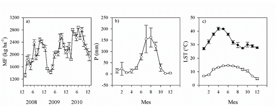
Figure 1 Environmental variables and production of a mixed alfalfa-grass mixed pasture grazed by beef cattle: a) forage mass (FM), b) rainfall (P) and c) diurnal (●) and nocturnal (○) surface temperature (LST)
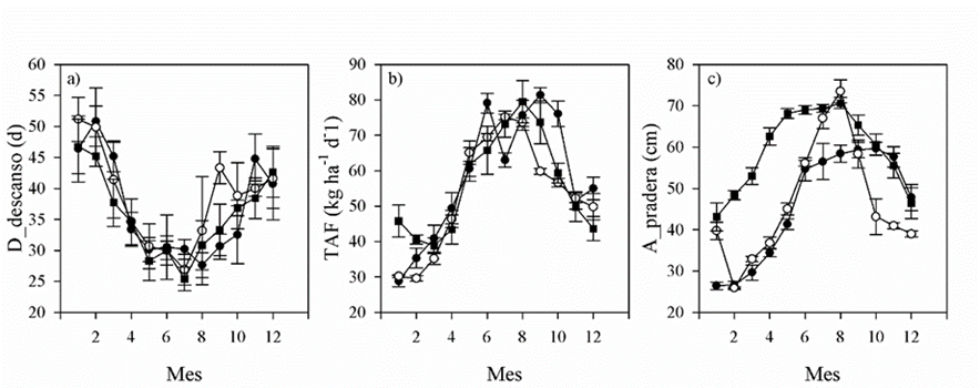
Figure 2 Management of a mixed alfalfa-grass mixed pasture grazed by beef cattle during 2008 (●), 2009 (○) and 2010 (■): a) Rest days before grazing, b) rate of accumulation of forage (PAR) of the period, c) pasture height
In MA regression, the intercept was numerically close to 0 in the ML_RS_PM scenario and its slope was equal to 1, a model with slope equal to 1 and intercept equal to 0 indicates good fit. The lower value of the RMSE, AIC, BIC and deviance suggested a better representation of the FM with the ML_RS_PM scenario (Table 1). Regarding deviance analysis, the comparison between two or more models will be valid if they fit the same data set, this requirement was not met because the predicted values of FM were inherently different for each model generated. The difference of deviances is distributed approximately as X2 with degrees of freedom equal to the difference in the number of parameters between the models14, with this difference being 0 for the case of simple linear regression models used to represent the relationship between estimated and predicted values in each modeling scenario. For these two reasons, deviance analysis was not possible; therefore, the selection of the best model was based solely on the numerical value of the goodness-of-fit measures. The worst model was the simple regression between FM and H_pasture, not only according to the goodness-of-fit means but also in the graphical representation of the estimated vs. observed values (Figure 3).
Table 1 Goodness-of-fit measures between observed and estimated FM values resulting from modeling scenarios using algorithms of ordinary least squares (OLS) or machine learning (ML) in combination with explanatory variables related to pasture management (PM) alone or in conjunction with remote sensing variables (PM_RS)
| OLS_height | OLS_RS | OLS_RS_PM | ML_RS | ML_RS_PM | |
|---|---|---|---|---|---|
| r2 | 0.40 | 0.49 | 0.67 | 0.70 | 0.97 |
| RMSE | 361.0 | 341.0 | 269.0 | 259.0 | 78.0 |
| AIC | 734.0 | 724.0 | 686.0 | 691.0 | 542.0 |
| BIC | 738.0 | 728.0 | 690.0 | 695.0 | 546.0 |
| Deviance | 8079684.0 | 6874194.0 | 4377078.0 | 4003784.0 | 363954.0 |
| Bias | -3.4 | 47.1 | 16.5 | -35.1 | -1.3 |
| CI 2.5 % | -95.9 | -39.2 | -52.7 | -43.5 | -21.2 |
| CI 97.5 % | 89.0 | 133.5 | 85.7 | 96.4 | 18.6 |
| MA intercept | -1799.0 | -2044.0 | -594.0 | -735.0 | 27.0 |
| CI 2.5 % | -3386.0 | -3395.0 | -1137.0 | -1257.0 | 62.0 |
| CI 97.5 % | -831.0 | -1162.0 | -162.0 | -316.0 | 112.0 |
| MA slope | 1.9 | 2.0 | 1.3 | 1.4 | 1.0 |
| CI 2.5 % | 1.4 | 1.6 | 1.1 | 1.2 | 0.9 |
| CI 97.5 % | 2.6 | 2.7 | 1.6 | 1.6 | 1.0 |
r2= coefficient of determination; RMSE= root mean square error; AIC= Akaike information criterion; BIC= Bayesian information criterion; MA= major axis regression; CI= confidence interval.
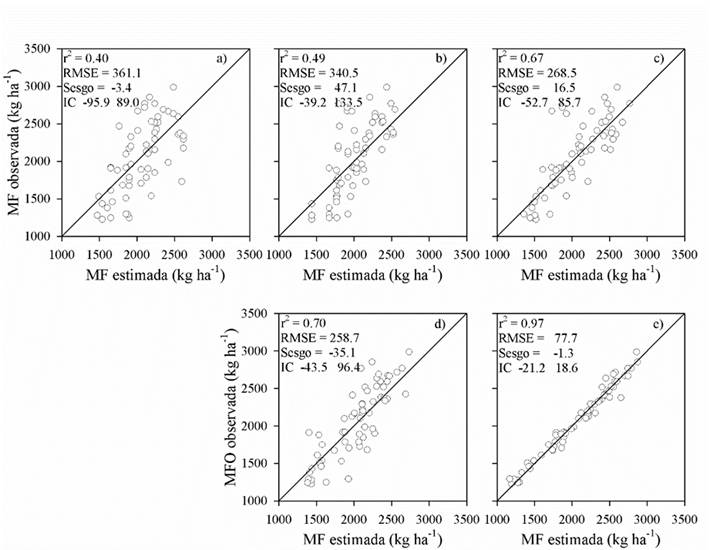
a) OLS, predictor variable forage height; b) OLS_RS scenario; c) OLS_RS_PM scenario; d) ML_RS scenario; e) ML_RS_PM scenario. Coefficient of determination (r2), root mean square error (RMSE), bias and its 95 % confidence interval (CI=IC).
Figure 3 Evaluation between observed and estimated values of FM using algorithms of ordinary least squares (OLS) or machine learning (ML)
The PAR and H_pasture variables of PM were the most important (Table 2), both in the ML and OLS models; the variable R_time was much less important (Table 2). The most important RS variables were: LST_n, P, P_lag_3 or P_lag_5, LST_d_avg_3 or LST_n_avg_3; indicating the relevance of the environmental conditions of precipitation and temperature not only of the current month, but of the conditions preceding the measurement of the FM. Reflectance (b1 - b7) and vegetation indices were incorporated into ML models, but the stepwise procedure did not choose them for OLS. Compared with PAR and H_pasture, reflectance variables were of low importance in the RS_PM scenarios of ML. Spectral reflectance bands were more important than EVI and NDVI; this finding coincides with the FM study for mixed pastures of temperate climate15. Although the prediction of fresh biomass in Brachiaria pastures based on the NDVI with r2= 0.7331 was considered adequate.
Table 2 Important variables included in the scenarios using two possible algorithms: ordinary least squares (OLS) or machine learning (ML) and two types of explanatory variable: only remote sensors (RS) or pasture management variables and RS (RS_PM)
| Variable | Machine learning (ML) |
Ordinary least squares (OLS) | ||
|---|---|---|---|---|
| Remote sensors (RS) |
Remote sensors (RS)_Pasture management (PM) |
RS | RS_PM | |
| LST_d_avg_3 | 0.081 | 0.023 | 0.036 | 0.027 |
| LST_n_avg_3 | 0.064 | 0.017 | ||
| LST_d | 0.036 | 0.036 | ||
| LST_n | 0.161 | 0.007 | 0.060 | |
| b1 | 0.027 | 0.008 | ||
| b2 | 0.034 | 0.014 | ||
| b3 | 0.028 | 0.003 | ||
| b4 | 0.033 | 0.004 | ||
| b5 | 0.044 | 0.008 | ||
| b6 | 0.048 | 0.010 | ||
| b7 | 0.096 | 0.008 | ||
| P | 0.058 | 0.008 | 0.048 | |
| P_lag_3 | 0.099 | 0.023 | ||
| P_lag_5 | 0.270 | |||
| NDVI | 0.001 | |||
| EVI | 0.018 | 0.001 | ||
| H_pasture | 0.303 | 0.231 | ||
| Month_beg_grow | 0.006 | 0.020 | ||
| R_time | 0.101 | 0.072 | ||
| PAR | 0.417 | 0.368 | ||
For ML models the sum of importance is 1, for OLS models the sum of importance is equal to the r2.
The partial dependence that existed between the prediction of FM and the value of some of the most important variables in some ML models is shown in Figure 4, in the ML_RS scenario and in Figure 5 for the ML_RS_PM scenario. The ensembles of ML models had lower deviance compared to some ML algorithms in the two scenarios and were therefore considered better representations of the FM. The partial dependence figures indicate how the explanatory variable influences the predictions of one of the models or ensembles, after standardizing the effect of other variables. For linear regression models (such as the GLM model obtained by ML), the figure is a straight line with slope equal to the parameter of the model32. FM depended directly and proportionally on the variables PAR, H_pasture and R_time in different models even for a GLM model (pink line), but for variables P_lag_3 and LST_d, the dependence differed between the GLM model and ML models, particularly the DL-type model (dark green line) which was the best individual ML model (Figure 5). The interpretation of the figures is improved with the frequency histogram of the observations, depending on the value of the variable. Where there was less frequency of data, it was interpreted that dependence was not supported by sufficient evidence. An example of this situation was the dependence of LST_n in Figure 4, where the DL-type model has an abrupt ascent, but the last two class intervals of the histogram have few observations.
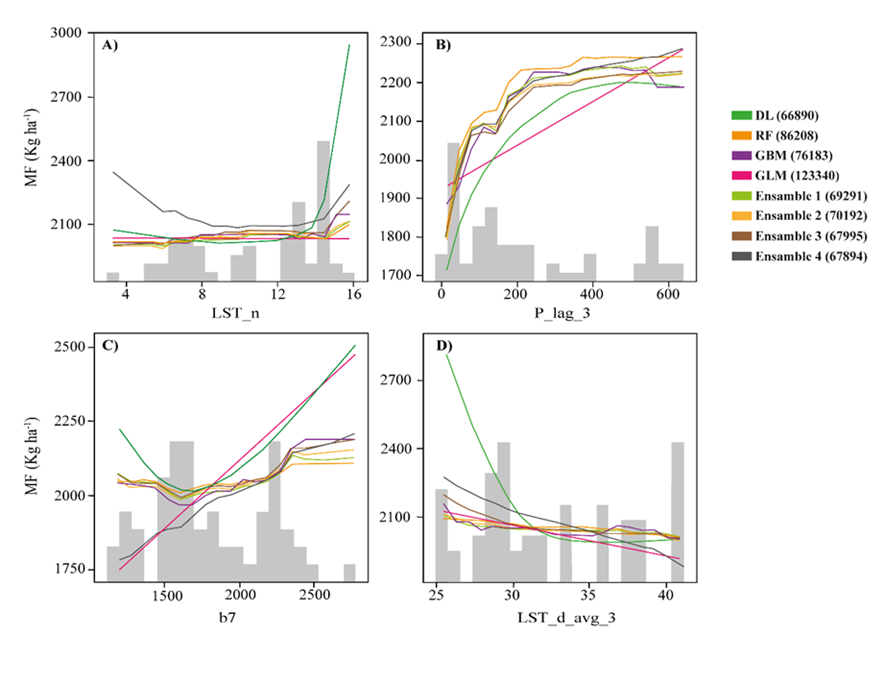
The gray bars are the data frequency according to class intervals of the variable. Only models of lower deviance (value in parentheses) obtained by machine learning in the scenario using only variables measured with remote sensors (ML_RS) are shown.
Figure 4 Partial dependence of FM and: A) monthly average of nocturnal surface temperature (LST_n), B) precipitation accumulated in the previous three months (P_lag_3), C) reflectance band b7 of the MODIS MCD43A4 product, D) monthly average of the diurnal surface temperature in the previous three months (LST_d_avg_3)
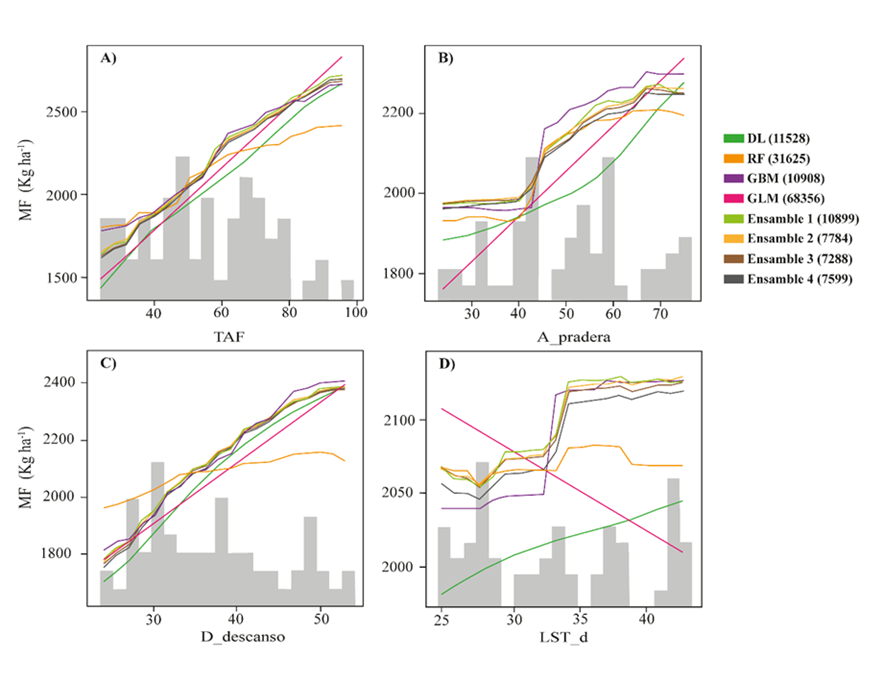
The gray bars are the data frequency according to class intervals of the variable. Only models of lower deviance (value in parentheses) obtained by machine learning in the scenario using variables measured with remote sensors and of pasture management (ML_RS_PM) are shown.
Figure 5 Partial dependence of FM and: A) rate of accumulation of forage (PAR), B) forage height (H_pasture), C) pasture rest days (R_time), D) monthly average of the diurnal surface temperature (LST_d)
The ML_RS_PM scenario included the PAR variable, and this could be a limitation for the practical application of the model. To clarify this aspect, an ML model was built without this variable and using the same training data, resulting in an r2 of 0.76, RMSE of 232.2 and bias of -35.6 (CI -94.4 to 23.1), being better than that obtained in the ML_RS scenario (data not shown). This result has two aspects of importance: other variables available for modeling can replace a variable identified as the most important and second, it is possible to incur into a local optimal solution, even when the ML algorithm explored a solution space with different optimization parameters. A possible alternative would be to increase the number of times the h2o.automl function is run and increase the value of the max_runtime_secs constant.
Despite the coarse spatial resolution of the MODIS and GPM remote sensors (250 m2 and 10 km2), the FM was adequately estimated in the ML_RS scenario (Figure 3d), the r2= 0.70 of this model was within the range recently reported in the literature for ML models that estimate biomass with RS data14,15 or gross primary productivity33. A model based on RS data is only attractive for the management of large grasslands. When RS variables were used in combination with pasture management variables that are easy to measure (H_pasture) or record (R_time and Month_beg_grow), the estimate was very good (Figure 3e); the r2= 0.97 was similar to the r2= 0.96 of biomass estimated from 30 m spatial resolution RS data5. The prediction of the forage mass obtained with forage height measurements improved when pasture management variables and local meteorological data were incorporated into an ML algorithm of random forest (r2= 0.82), this approach was judged practical for producers, albeit the cost of meteorological instruments2.
Despite being an irrigated pasture, the previous short-term rain was important information for OLS and ML models. In a recent study, it was identified that the spatial-temporal variation of gross primary productivity was not only explained by reflectance bands of the MODIS MCD43A4 but was also related to the vapor pressure deficit33. Similar to the result of these authors, here it was useful to include other reflectance bands besides b1, b2 and vegetation indices such as NDVI and EVI. From a practical point of view, the model of the ML_RS_PM scenario was considered very feasible to implement as it used routine measurements of the management of the pasture and NASA’s remote sensor data which are publicly accessible.
Animal production under grazing is sustainable when feed consumption that meets nutrient needs is ensured. In grazing management, this depends on adjusting the stoking rate according to the phenological stage of the plant, to the FM before and after grazing and to the forage that is decided to leave as residual pasture mass. For beef cattle, adequate FM before grazing can be set at 2,500 kg ha-1 and FM after grazing around 1,200 kg ha-110; although these thresholds will depend on the reproductive and physiological stage of the animal, the season of year and different pasture management strategies for feed rationing, phenological control or balance in botanical composition34. For these reasons, it is important that the predictive model of FM fits well at the extremes of its range and with the exception of the ML_RS_PM scenario, there was an overestimation of the FM when it was less than approximately 1,500 kg ha-1 (Figure 3).
Pasture mass is spatially variable given by differences in soil moisture and fertility, dung deposition, alterations in the plant community by selective grazing and other factors. Forage quadrant cuttings are limited to represent and capture this spatial variability in pastures and therefore the statistical method of sampling is important. Sensors on board unmanned aerial vehicles or drones are an alternative to capture variability in vegetation reflectance on the spatial scale of centimeters, but the cost of multispectral equipment, data processing and operational limitation to cover the territory 35, in addition to the need for a calibration function for forage mass, must be considered.
Conclusions and implications
The prediction of FM had lower bias with ML models than with OLS models, especially when remote sensors and pasture management variables were incorporated in the models. ML ensembles had lower deviance compared to some of the individual ML models. The use of RS variables predicted FM similarly to the relationship between H_pasture and FM, although the ML model had lower bias. The models explored would have to be tested in other pasture conditions in order to have a spatial application, be able to represent ecosystems and to value the environmental service of carbon capture. At the local farm scale, these models could be applicable for everyday use in farm feed budgeting or retrospective evaluation of farm pasture management. In these cases, the results presented here are promising.
Acknowledgements
The study was the product of the support for sabbatical leave of the first author by the Autonomous University of Querétaro.
REFERENCES
1. Sheath GW, Hay RJM, Giles KH. Managing pastures for grazing animals. In: Nicol, AM, editor. Livestock feeding on pasture. NZ Soc Anim Prod occasional publication. 1987;65-74. [ Links ]
2. Murphy D, O’Brien B, Hennessy D, Hurley M, Murphy M. Evaluation of the precision of the rising plate meter for measuring compressed sward height on heterogeneous grassland swards. Precis Agric 2021;22(3):922-946. [ Links ]
3. Radcliffe J. Cutting techniques for pasture yields on hill country. Proc NZ Grassland Association. 1971;33:91-104. [ Links ]
4. Jáuregui JM, Delbino FG, Bonvini MIB, Berhongaray G. Determining yield of forage crops using the Canopeo mobile phone app. J NZ Grassl 2019;41-46. [ Links ]
5. Marsett RC, Qi J, Heilman P, Biedenbender SH, Watson MC, Amer S, et al. Remote sensing for grassland management in the arid southwest. Rangel Ecol Manag 2006;59(5):530-540. [ Links ]
6. O’Donovan M, Dillon P, Rath M, Stakelum G. A comparison of four methods of herbage mass estimation. Ir J Agric Food Res 2002;17-27. [ Links ]
7. Mills A, Smith M, Moot DJ. Relationships between dry matter yield and height of rotationally grazed dryland lucerne. J NZ Grassl 2016;(78):185-196. [ Links ]
8. Moot DJ, Yang X, Ta HT, Brown HE, Teixeira EI, Sim RE, et al. Simplified methods for on-farm prediction of yield potential of grazed lucerne crops in New Zealand. NZ J Agric Res 2021;65(4-5)1-19. [ Links ]
9. Robertson S. Mass to height relationships in annual pastures and prediction of sheep growth rates. Anim Prod Sci 2014;54(9):1305-1310. [ Links ]
10. Nicol AM, Nicoll GB. Pastures for beef cattle. In: Nicol, AM. editor. Feeding livestock on pasture. Society of Animal Production. Lincoln, New Zealand. 1987;119-131. [ Links ]
11. Zhang Y, Ye A. Would the obtainable gross primary productivity (GPP) products stand up? A critical assessment of 45 global GPP products. Sci Total Environ 2021;783:146965. [ Links ]
12. Jiao W, Wang L, McCabe MF. Multi-sensor remote sensing for drought characterization: current status, opportunities and a roadmap for the future. Remote Sens Environ 2021;256:112313. [ Links ]
13. Anav A, Friedlingstein P, Beer C, Ciais P, Harper A, Jones C, et al. Spatiotemporal patterns of terrestrial gross primary production: A review. Rev Geophys 2015;53(3):785-818. [ Links ]
14. Lang M, Mahyou H, Tychon B. Estimation of rangeland production in the arid oriental region (Morocco) combining remote sensing vegetation and rainfall indices: challenges and lessons learned. Remote Sens 2021;13(11):2093. [ Links ]
15. Chen Y, Guerschman J, Shendryk Y, Henry D, Harrison MT. Estimating pasture biomass using sentinel-2 imagery and machine learning. Remote Sens 2021;13(4):603. [ Links ]
16. Hacker R, Smith W. An evaluation of the DDH/100 mm stocking rate index and an alternative approach to stocking rate estimation. Rangel J 2007;29(2):139-148. [ Links ]
17. CICESE C de IC y de ES de E. Base de datos climatológica nacional (CLICOM). [Internet]. Tequisquiapan, Querétaro; 2021. Estación 22025: Consultada 6 Mar, 2021. http://clicom-mex.cicese.mx/ . [ Links ]
18. Hodgson J. Grazing management. Science into practice. Longman Group UK Ltd. 1990. [ Links ]
19. Schaaf C, Wang Z. MCD43A4 MODIS/Terra+ Aqua BRDF/Albedo Nadir BRDF Adjusted Ref Daily L3 Global 500 m V006. NASA EOSDIS Land Processes DAAC. 2015. [ Links ]
20. R Development Core Team. R: A language and environment for statistical computing. R Foundation for Statistical Computing. 2009. https://www.r-project.org [ Links ]
21. QGIS.org. QGIS Geographic Information System. QGIS Association. 2021. http://www.qgis.org [ Links ]
22. Google maps. Mapa satelital. México; 2021. [ Links ]
23. Pasquel D, Roux S, Richetti J, Cammarano D, Tisseyre B, Taylor JA. A review of methods to evaluate crop model performance at multiple and changing spatial scales. Precis Agric 2022;23:1489-1513. [ Links ]
24. Warton DI, Duursma RA, Falster DS, Taskinen S. smatr 3-an R package for estimation and inference about allometric lines. Methods Ecol Evol 2012;3(2):257-259. [ Links ]
25. Tedeschi LO. Assessment of the adequacy of mathematical models. Agric Syst 2006;89(2):225-247. [ Links ]
26. Hall P, Gill N, Kurka M, Phan W, Bartz A. Machine learning interpretability with H2O driverless AI. Bartz A. Editor. California, U.S.: H2O.ai Inc.; 2019. [ Links ]
27. LeDell E, Poirier S. H2o automl: Scalable automatic machine learning. In 2020. https://www.automl.org/wp-ontent/uploads/2020/07/AutoML_2020_paper_61.pdf. [ Links ]
28. Mitchell R, Frank E. Accelerating the XGBoost algorithm using GPU computing. PeerJ Comput Sci 2017;3:e127. [ Links ]
29. McElreath R. Statistical rethinking: A bayesian course with examples in R and STAN. Boca Raton, FL. U.S.: CRC Press; 2020. [ Links ]
30. Wang J, Petersen WA, Wolff DB. Validation of satellite-based precipitation products from TRMM to GPM. Remote Sens 2021;13(9):1745. [ Links ]
31. Bretas IL, Valente DS, Silva FF, Chizzotti ML, Paulino MF, D’Áurea AP, et al. Prediction of aboveground biomass and dry‐matter content in Brachiaria pastures by combining meteorological data and satellite imagery. Grass Forage Sci 2021;76(3):340-352. [ Links ]
32. Friedman JH. Greedy function approximation: a gradient boosting machine. Ann Stat 2001;1189-1232. [ Links ]
33. Joiner J, Yoshida Y. Satellite-based reflectances capture large fraction of variability in global gross primary production (GPP) at weekly time scales. Agric For Meteorol 2020;291:108092. [ Links ]
34. Griffiths W, Dodd M, Kuhn-Sherlock B, Chapman D. Management options to recover perennial ryegrass populations and productivity in run-out pastures. NZGA: Research and Practice Series. 2021;17. [ Links ]
35. Ahmad A, Ordonez J, Cartujo P, Martos V. Remotely piloted aircPARt (RPA) in agriculture: A pursuit of sustainability. Agronomy 2021;11(1):7. [ Links ]
Received: March 08, 2022; Accepted: July 18, 2022
 Este es un artículo publicado en acceso abierto bajo una licencia Creative Commons
