


 texto en
  Inglés (pdf)
 Artículo en XML
 Referencias del artículo
 Enviar artículo por email
 Citado por SciELO
  Similares en
SciELO
Similares en
SciELO 
 Permalink
Introduction
Mexican Braunvieh is a dual-purpose breed of cattle. Since June 2003, national genetic evaluations for growth traits have been undertaken for this breed in Mexico1. Like in any livestock population, there are unknown parents in the pedigree. Unknown parents are assumed to be unrelated, non-inbred, and to have a single descendant. Unknown parents might correspond to base animals in the first generation or spread over generations. They affect genetic progress in several ways: (i) reducing selection intensity for animals with unknown parents, (ii) parentage uncertainty decreases the accuracy of genetic evaluations, (iii) miss-identification of parents yields both biased estimated breeding values (EBV) and heritability estimates2. Best linear unbiased prediction (BLUP) regresses genetic merit predictions of animals to unknown parents of mean zero. Depending on the genetic background, and the generation to which unknown parents belong to, their expected genetic merit could be different from zero. Quass3 established a methodology for considering phantom parent groups (PPG) or genetic groups in BLUP. Although PPG are not of interest per se, they are considered to facilitate modeling and computation4. Furthermore, along with statistical correction for non-random missing pedigree information, PPG enables direct estimation of quantitative genetic parameters5.
Because there are no specific rules for determining PPG, its definition is mainly based on the researcher’s criteria, but it usually includes a time component6. Other factors commonly considered in grouping strategies are the sex of the parent or selection intensity4,7,8. All descendants of an individual with PPG contribute to the estimation of the PPG effect5, so having PPG with an equal number of individuals is unlikely to affect the animal model’s ability to estimate the PPG effect with acceptable precision. However, any strategy for assigning unknown parents to PPG should reflect the average genetic level of unknown parents9.
Due to the inclusion of PPG in the model, Theron et al7 observed a significant change and a reduction of bias in the genetic trend of milk yield for South African Holsteins. Similarly, a reduction in EBV bias was detected by including PPG in the genetic analyses for weaning, post-weaning and yearling weights, scrotal circumference, and muscling score in Nelore cattle10. The purpose of this study was to compare two strategies of grouping unknown parents to PPG on the genetic evaluation of growth traits in Mexican Braunvieh cattle.
Material and methods
Data
Pedigree and phenotypic records on Mexican Braunvieh cattle were obtained from Asociación Mexicana de Criadores de Ganado Suizo de Registro (Mexico City). Phenotypic records were birth (BW), weaning (WW), and yearling weights (YW) from animals born between 1985 and 2017, in 229 farms across Mexico. Weaning and yearling weights were adjusted to 240 d and 365 d of age, respectively, according to the procedure proposed by the Beef Improvement Federation11. Records outside the mean ± 3 SD range for the trait of interest were not included in the analyses. Also, WW and YW records outside 240 ± 45 d and 365 ± 45 d age were excluded from the analyses, respectively. The pedigree was extracted (parents), starting from animals with an available phenotype (for any of the three traits), and limited to animals born since 1970. Final pedigree included 57,341 individuals, 18,689 males, 38,652 females, 2,746 sires, and 27,015 dams.
Contemporary groups were formed considering herd, year, and season of birth (rainy or dry). Records from contemporary groups with less than four animals were excluded from the analyses. Table 1 shows the final number of records and descriptive statistics for each trait.
Genetic analyses
The genetic analyses comprised estimation of genetic parameters and BLUP12 for the Mexican Braunvieh population, using the following single-trait models:
for BW and YW, and
for WW, where y, b, u, m, mpe, and e are vectors of phenotypic records, fixed effects, direct additive genetic, maternal additive genetic, maternal permanent environmental, and residuals effects, respectively. X, Z 1, Z 2, and Z 3 are incidence matrices relating records to b, u, m, and mpe, respectively. The fixed effects were:
bBW = [sex, Braunvieh purity, age of dam, (age of dam)2, birth contemporary group]
bWW = [sex, Braunvieh purity, age of dam, (age of dam)2, pre-weaning contemporary group, milk feeding condition]
bYW = [sex, Braunvieh purity, post-weaning contemporary group, post-weaning feed]
There were 1,778, 1,450, and 1,038 birth contemporary groups, pre-weaning contemporary groups, and post-weaning contemporary groups, respectively. Milk feeding conditions were suckling without milking, suckling with additional milking, and feeding with a milk substitute. Post-weaning feed regimes were grazing, semi-confined, and total confinement. The sex ratios were close to 1. Age of dam at calving had a minimum, mean, SD, and maximum of 1.70, 6.64, 3.04, and 17.00 yr, respectively. Braunvieh purity had a minimum, mean, SD, and maximum of 0.88, 0.99, 0.01, and 1.00, respectively. It was used the official models for the evaluation of the studied traits in Mexican Braunvieh cattle. The (co)variance structures were:
for BW and YW, and
for WW, where A is the pedigree-based additive genetic relationship matrix, I
Nd
and I
N
are identity matrices of order equal to the number of dams and observations.
Genetic groups
Evaluation of the genetic grouping strategies was carried out through the comparison of EBV from BLUP with and without PPG. Criteria used to form unknown parents’ groups were:
1) Year of birth: Year of birth of the unknown parent was five years before the year of birth of its progeny. Unknown parent birth years were grouped into six classes: 1965-69, 1970-74, 1975-79, 1980-84, 1985-89, and 1990-96.
2) Sex of the unknown parent.
3) Selection pathway (sire of sire, sire of dam, dam of sire, and dam of dam).
The two genetic grouping strategies were:
G12: Class of birth year (6 levels) × sex of the unknown parent (2 levels).
G24: Class of birth year (6 levels) × pathway of selection (4 levels).
Genetic groups based on criteria such as sex of missing ancestor or paths of selection allow evaluation of different genetic selection differentials4. Likewise, the inclusion of the year of birth category allows us to model the genetic improvement over time3,7. Table 2 shows the number of unknown parents in each PPG for each strategy.
Table 2 Criteria and frequency of unknown parents in phantom parent groups
| Strategy1 | Unknown parent |
Year group2 | |||||
|---|---|---|---|---|---|---|---|
| 1965- 1969 |
1970- 1974 |
1975- 1979 |
1980- 1984 |
1985- 1989 |
1990- 1996 |
||
| G12 | Sire | 540 | 513 | 820 | 941 | 678 | 433 |
| Dam | 647 | 457 | 664 | 891 | 564 | 35 | |
| G24 | Sire of sire | 119 | 58 | 72 | 90 | 87 | 143 |
| Sire of dam | 421 | 455 | 748 | 851 | 591 | 290 | |
| Dam of sire | 145 | 57 | 51 | 84 | 73 | 9 | |
| Dam of dam | 502 | 400 | 613 | 807 | 491 | 26 | |
1 Phantom parent group with 12 (G12) and 24 (G24) levels.
2 Progeny’s birth year - 5.
Without including PPG in the model, the mixed model equations were (for BW and YW):
where
Incorporating PPG effects into the genetic merit of animals (i.e., EBV = û + Qĝ) can be made directly in the mixed model equations, using Quaas and Pollak14 transformation that involves absorption of PPG equations, which gives3:
This procedure avoids the extra step of calculating û + Qĝ after Eq. [4], and the need for re-creating matrix Q, which is computationally expensive. Quaas and Pollak14 transformation is not implemented in MTDFREML software. Therefore, Eq. [3, 4] were applied for BLUP with and without PPG, respectively (additional terms of the maternal genetic and maternal permanent environmental effects were involved for WW). Estimated breeding values accounting for PPG (û + Qĝ) were obtained using functions “qmat” and “Qgpu” from R package “ggroups”15, where the matrix of PPG contributions to individuals in a pedigree (Q) was calculated, and PPG contributions (Qĝ) were added to the genetic merit of animals (û), with ĝ and û obtained from MTDFREML13.
Results and discussion
There were 3,925 animals with unknown sire, 3,258 animals with unknown dam, and 2,430 animals with both unknown sire and dam. Unknown parents were assigned to 12 or 24 PPG (G12 and G24; Table 2). Variance components obtained with and without PPG are shown in Table 3. Estimates of parameters for the studied traits under different scenarios were closely similar. Thus, the model choice should not interfere with the estimation of genetic parameters.
Table 3 Variance components for birth weight (BW), weaning weight (WW) and yearling weight (YW) for the Mexican Braunvieh population estimated with 12 (G12), 24 (G24) and without (G0) phantom parent groups
| Strategy | Trait |
|
|
|
|
|---|---|---|---|---|---|
| G0 | BW | 2.69 | - | - | 8.54 |
| WW | 87.76 | 8.80 | 23.12 | 435.85 | |
| YW | 86.27 | - | - | 692.96 | |
| G12 | BW | 2.69 | - | - | 8.53 |
| WW | 83.14 | 8.43 | 23.06 | 436.58 | |
| YW | 81.30 | - | - | 695.01 | |
| G24 | BW | 2.71 | - | - | 8.52 |
| WW | 90.27 | 10.09 | 21.37 | 435.37 | |
| YW | 85.72 | - | - | 692.52 |
Theron et al7 reported that the inclusion of PPG has a minor influence on the estimation of co(variance) components, also, Shiotsuki et al16 showed that the use of a relationship matrix that includes genetic groups does not generate differences in the variance estimates contrasted with the use of a matrix without genetic groups. In some studies7,8,10 variance components were obtained considering a "control" model, which did not include genetic groups, and those variance components were used in predicting breeding values in a model including PPG, similar to the procedure applied in this research.
Descriptive statistics for EBV obtained with models including or excluding PPG are shown in Table 4. In a basic animal model, the existence of a single genetic group is assumed17. Given that breeding values are deviations from the genetic group mean, all values in the base population have an expectation of zero5,17. Genetic group methodology allows to assign genetic effects to multiple groups within the base population, which could have a different mean5. The EBV including genetic groups considers that each individual inherits the mean of the effects in the genetic group of their parents plus the mean of the genetic value of their parents; therefore, the expectation of EBV for the population is not zero5,17 because the assumption of breeding values distribution is not met. Assigning unknown parents to PPG with a possibly non-zero average of genetic merit would change their descendants’ EBV. Consequently, the expected mean of the EBV obtained after considering genetic groups change to the product Qg3.
Table 4 Descriptive statistics of estimated breeding values for growth traits obtained with 12 (G12), 24 (G24) and without (G0) phantom parents groups for Mexican Braunvieh cattle
| Strategy | Trait | Minimum | Mean ± SD | Maximum |
|---|---|---|---|---|
| G0 | BW | -5.36 | 0.03 ± 0.79 | 5.13 |
| WW | -26.67 | -0.17 ± 3.87 | 25.32 | |
| YW | -24.06 | 0.32 ± 3.39 | 24.34 | |
| G12 | BW | -5.24 | 0.31 ± 0.83 | 5.37 |
| WW | -18.73 | 14.19 ± 5.20 | 39.77 | |
| YW | -50.60 | -7.77 ± 4.81 | 18.08 | |
| G24 | BW | -3.67 | 2.06 ± 0.88 | 7.57 |
| WW | -53.15 | -10.75 ± 8.17 | 32.23 | |
| YW | -49.13 | 31.10 ± 7.27 | 82.12 |
BW= Birth weight, WW= Weaning weight, YW= Yearling weight.
Pearson product-moment and Spearman rank correlations between EBV with and without PPG are shown in Table 5. Correlation coefficients between EBV without PPG (G0) and G12 were higher than those of G0 and G24, for all the traits and groups of animals (i.e., males and females, with and without phenotype). The correlations were lower for animals without phenotype than with phenotype, and lower for females than males. Generally, the correlations were higher for BW than for WW, and higher for WW than for YW (Table 5).
Table 5 Pearson(and Spearman) correlation coefficients between estimated breeding values without phantom parent groups (EBV_G0), with 12 phantom parent groups (EBV_G12), and 24 phantom parent groups (EBV_G24), in the Mexican Braunvieh population
| Correlation type | Trait | ||
|---|---|---|---|
| Birth weight | Weaning weight | Yearling weight | |
| Total animals | n =57,341 | n = 57,341 | n = 57,341 |
| r(EBV_G0, EBV_G12) | 0.959 (0.942) | 0.766 (0.766) | 0.692 (0.717) |
| r(EBV_G0, EBV_G24) | 0.912 (0.891) | 0.538 (0.610) | 0.535 (0.605) |
| Males with phenotype | n = 15,810 | n = 10,748 | n = 7,384 |
| r(EBV_G0, EBV_G12) | 0.988 (0.982) | 0.914 (0.886) | 0.853 (0.846) |
| r(EBV_G0, EBV_G24) | 0.975 (0.964) | 0.786 (0.763) | 0.743 (0.737) |
| Males without phenotype | n = 2,879 | n = 7,941 | n = 11,305 |
| r(EBV_G0, EBV_G12) | 0.941 (0.923) | 0.796 (0.797) | 0.719 (0.760) |
| r(EBV_G0, EBV_G24) | 0.861 (0.830) | 0.606 (0.627) | 0.587 (0.636) |
| Females with phenotype | n = 15,844 | n = 10,585 | n = 7,055 |
| r(EBV_G0, EBV_G12) | 0.986 (0.979) | 0.901 (0.879) | 0.844 (0.840) |
| r(EBV_G0, EBV_G24) | 0.972 (0.960) | 0.752 (0.749) | 0.710 (0.743) |
| Females without phenotype | n = 22,808 | n = 28,067 | n = 31,597 |
| r(EBV_G0, EBV_G12) | 0.895 (0.877) | 0.635 (0.659) | 0.596 (0.634) |
| r(EBV_G0, EBV_G24) | 0.799 (0.781) | 0.407 (0.491) | 0.445 (0.515) |
It has been proposed that correlation coefficients between EBV lower than 0.90 could change the ranking of animals for genetic evaluation18. Estimates of correlation coefficients obtained here suggest possible changes in the ranking mainly for WW and YW. Petrini et al8 also remarked changes in the rank for WW due to the inclusion of PPG (Pearson and Spearman correlation estimates ranged from 0.50 to 0.70). On the other hand, the inclusion of PPG resulted in small changes in the ranking for BW in this study. Results for BW agree with what was observed for milk production7, YW, and post-weaning weight gain16, scrotal circumference, or muscle score8. Rank changes are due to the shifts that genetic groups make in the EBV of their descendants.
Figure 1 illustrates the effect of PPG on genetic trends. The trends were relatively similar for males and females. For BW, G12 increased the slope of the genetic trend, compared to G0; G24 also increased the slope of the genetic trend, but it showed a base deviation from G0. For WW, both G12 and G24 showed large fluctuations in the early years. Genetic trends from G12 and G24 showed positive and negative base differences with G0, respectively (Figure 1). For YW, the genetic trend of G24 showed a large base deviation from the G0 and G12 genetic trends (Figure 1). Generally, if a genetic trend does not pass over zero, it indicates a base problem for EBVs. Therefore, G24 is ruled out for BW and YW, and G12 is ruled out for WW, since G24 does not cross zero for BW and YW, and G12 does not cross zero for WW (Figure 1). On the other hand, a robust grouping strategy is expected to perform well for different traits16, as a trait-specific grouping strategy would be a burden for routine genetic evaluations.
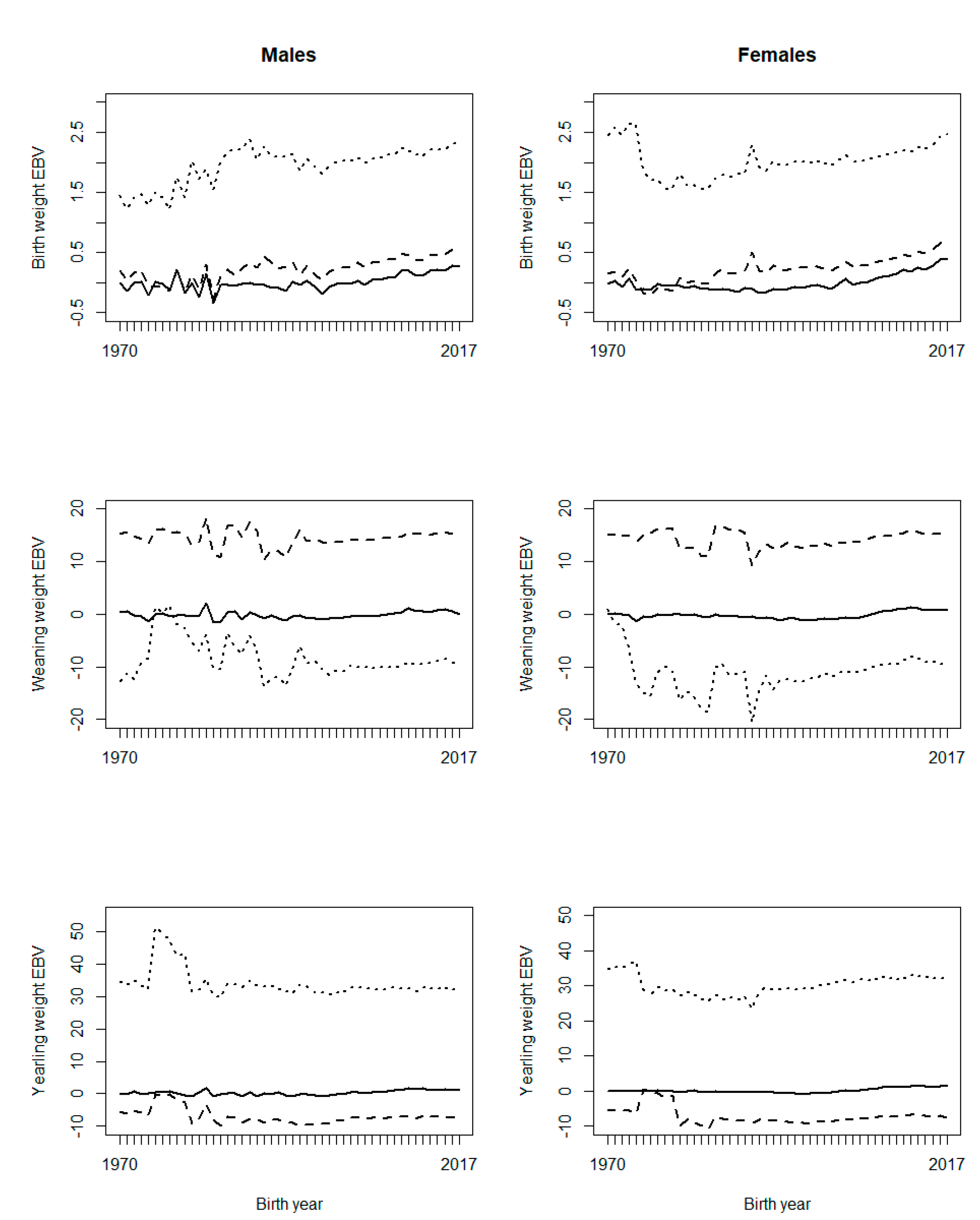
Figure 1 Genetic trends of growth traits for BLUP (EBV (solid line)), BLUP with 12 phantom parent groups (EBV_G12 (dashed line)), and BLUP with 24 phantom parent groups (EBV_G24 (dotted line)), with six classes of birth year considered in phantom parent groups
However, in practice, a grouping strategy may perform well for a trait, but not well for another trait, especially if the fixed effects are different for the two traits8. Possible problems with PPG implementation are likely to be due to collinearity or confounding between PPG and fixed effect3,5. Considering PPG as random effect is a solution to this problem.
The effect of inclusion of PPG on the genetic trend has been variable. Theron et al7 showed that including PPG in genetic evaluation had a drastic effect on the genetic trend for milk production traits, having a higher response (almost double) when PPG was included. Besides, Shiotsuki et al16 observed higher genetic trends for post-weaning weight and YW when the model included PPG. In contrast, PPG inclusion in genetic analyses for WW, scrotal circumference, and muscling score showed a lower genetic trend than when PPG was not included8. It could be concluded that the effectiveness of PPG on genetic evaluations depends on the population structure, studied traits and criteria adopted to define PPG. It has been proposed that the definition of PPG should balance between the complexity of genetic groups and the representation of genetic differences8. Also, genetic groups should consider the selection criteria adopted by breeders.
Two possible reasons are considered for the problems observed with the genetic trends: the shortage of progeny phenotypes supporting the inference of some PPG, and possible confounding or collinearity between PPG and the fixed effects in the model, especially contemporary groups. Figure 2 shows the frequency of animals, missing sires, and missing dams across birth years, and Figure 3 shows the frequency of phenotypes per birth year. It can be interpreted that there were not enough phenotypes supporting the prediction of PPG solutions in early years (unknown parents born before 1990, i.e., their progeny born before 1995). The phenotypes’ contribution decreases as the number of generations between the PPG and the phenotyped descendant increases, lower with lower heritability.
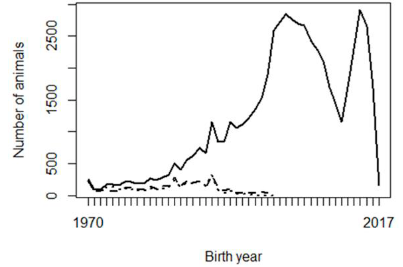
Figure 2 Number of animals (solid line), unknown sires (dashed line) and unknown dams (dotted line) per year of birth
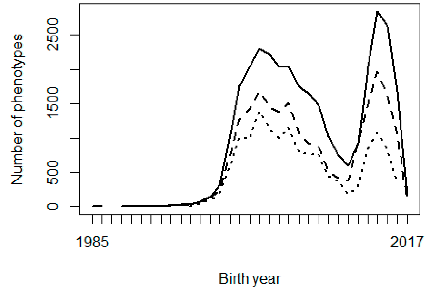
Figure 3 Number of birth weight (solid line), weaning weight (dashed line), and yearling weight (dotted line) phenotypes per year of birth
Figure 2 shows that the studied population was not in real need of PPG in the animal model, or PPG could be limited to only a few groups, so that phenotypes from distant generations of descendants could support the estimation of those few PPG. Animal models with PPG are more beneficial to populations with a higher and broader prevalence of missing pedigree information, especially if different genetic backgrounds (e.g., imported genetic materials) or different selection strategies/pressure are involved in different groups of animals (e.g., males vs. females or different selection pathways). The genetic trends (Figure 1) show that the population has not been under efficient selection, and there is an excellent opportunity for genetic improvement toward sustainable production in Mexican production systems and environments. Figures 2 and 3 also show data collection problems between years 2003 and 2014, and between 2014 and 2017. Data completeness and correctness are essential for accurate and reliable genetic evaluations.
As mentioned in the Data subsection, pedigree (parentage) was extracted, starting from phenotyped animals. The number of animals and missing parents (Figure 2) were higher without this restriction. However, in that case, there were extra missing parents with no contribution from progeny performance; therefore, no information to make inferences upon them. It is recommended to extract pedigree from phenotyped animals, making decisions about forming genetic groups, then adding animals that had not been extracted and assigning their unknown parents to the existing PPG.
Ideally, there should be fixed group connectedness between different PPG (i.e., like the concept of genetic connectedness among fixed groups (levels of a fixed effect)). In other words, phenotypes from different groups of fixed effects should contribute information to different PPG. It has even been recommended to form (some) PPG composite of both sires and dams8. The R package “ggroups”15 allows to perform PPG from both sexes. Similar definitions of PPG and some fixed effects may cause collinearity. In that situation, the number of fixed-effect groups contributing information to each PPG decreases. One way of checking the collinearity within and between fixed effects and PPG is checking the minimum eigenvalue of [X
Q
p]ʹ[X
Q
p], where Q
p is Q with rows limited to phenotyped animals. Estimability problems for PPG in the model are not limited to this study. Such problems are often observed due to confounded effects (collinearity) between PPG19. Even, reducing such confounding by changing the composition of PPG, there might be confounding between PPG and other fixed effects. Those estimability problems were removed and estimated breeding values look normal by considering PPG as random effects via adding
Conclusions and implications
Two strategies of grouping unknown parents to PPG (G12 and G24) were tested on BW, WW, and YW in Mexican Braunvieh cattle. The two strategies used the most common criteria for defining PPG (birth year of the progeny, sex of the unknown parent for G12, and selection pathway for G24). Genetic trends had an offset deviation from BLUP´s genetic trend without PPG, except for BW of G12. Also, including PPG in the model may have caused collinearity between PPG and some fixed effects. The shortage of phenotypes supporting the solutions for some PPG effects was another reason for the lack of benefit from the two grouping strategies on the studied population and traits. It is recommended to define PPG based on a subset of pedigree, in which parents are connected to phenotyped descendants, then adding the rest of animals and assigning their unknown parents to the existing PPG, to avoid an excessive and unnecessary number of genetic groups. More important than the number of progeny per PPG or equal year intervals defining PPG, is the amount of phenotype contributions for predicting PPG effects. It is recommended to have less overlap between PPG definitions and fixed effects to reduce collinearity between them.

