Introduction

In Mexico the Organization of the Sheep Breeders National Unit (Organismo de la Unidad Nacional de Ovinocultores - UNO) encompasses producers of specialized and pure breed sheep. This organization coordinates genetic improvement plans in sheep breeds based on genealogical records and production controls of the variables included in each breed’s selection criteria and objectives. Growth variables such as animal live weight are recorded at five points or ages¹. Live weight data for different ages is used to generate a points distribution over time. This allows analysis and characterization of growth patterns based on nonlinear mathematical models (NLM), which use biological interpretation to summarize variation in live weight over time through a small number of growth parameters and indicators^2,3.

Sheep production in Mexico occurs under various technological, agro-ecological and socioeconomic conditions. Organized and truthful documentation of events in the production unit, particularly financial variables, is essential for producers to determine unit profitability. Changes in animal live weight are influenced by genetic and environmental factors, with variable effects through time and during individual development. Each sheep breed has a characteristic growth pattern, requiring the testing of several NLM to identify that with the best fit for each breed. Identifying the NLM with the best fit provides objective and accurate growth pattern data which can be used by producers in decision-making regarding production, management and genetic improvement.

The present study objectives were: 1) To identify the best-fit NLM to describe the growth curve in four hair sheep breeds (Blackbelly, Pelibuey, Dorper and Katahdin) and three wool sheep breeds (Suffolk, Hampshire and Rambouillet); and, 2) To generate growth indicators that can characterize and analyze these growth curves.

Materials and methods

The analyzed database includes live weight records for female lambs in seven UNO-registered breeds: Blackbelly (BB), Pelibuey (PE), Dorper (DR), Katahdin (KT), Suffolk (SF), Hampshire (HS) and Rambouillet (RB). Analyzed variables were live weight at birth, 75, 120, 150 and 210 d of age, with measurements taken at intervals of ± 20 d with respect to the reference age (Table 1). Weight at 75 d corresponds to weaning. Because males are sold beginning at 120 d, only data for females was used in the analyses.

Data were from flocks mainly distributed in three regions of Mexico. Half (50 %) of the flocks were from the country’s central region and included primarily the SF, HS and RB breeds. The south-southeast region accounted for 22 % of the database, and corresponded to the PE, BB, DR and KT breeds. The north region represented 18 % of the data and included mostly the BB, DR and KT breeds. The remaining 10 % of the data was from flocks in other regions. Production systems in the central region are largely intensive or semi-intensive using stables combined with cultivated pastures. Systems in the north and south-southeast regions are semi-intensive and extensive, combining grazing with corrals. In the north, large arid and semi-arid areas with multispecies pastures and scrub are used, whereas in the south-southeast the tropical climate promotes wide availability of tropical grasses.

Seven NLM were evaluated: Brody (BRO), Verhulst (VER), von Bertalanffy (VBE), Gompertz (GOM), Mitscherlich (MIT) and logistic (LOG). All consisted of three regression coefficients (β₁, β₂ and β₃)^4,5,6. In NLM equations (Table 2), y _i represents live weight (kg) measured at time t ; β₁ is the asymptotic value when t tends to infinity, interpreted as the adult weight parameter (AW); β₂ is a fit parameter when y ≠ 0 and t ≠ 0; and β₃ is growth rate (GR), expressing weight gain as a proportion of total weight^2,7. The VER, VBE, GOM and LOG models describe growth based on a sigmoid curve, for which inflection point age (IPA) and weight (IPW) were estimated^8,9.

Analyses were done using the Gauss-Newton method of the NLIN procedure in the SAS statistical program¹⁰. Selection of the model with the best fit was done based on seven criteria^11,12,13: a) the Akaike information criterion [AIC = n*nl(sse/n) + 2k]; b) the Bayesian information criterion [BIC = n*nl(sse/n) + k*nl(n)]; c) the average prediction error [( APE=∑i=1nlwi - ewiewi*100 )/n]; d) the prediction error variance [ PEV =∑i=1n(ewi-lwi)2/n]; e) the Durbin-Watson statistic [DW= 2(1 - ρ); ρ= ∑t=2n(et-et-1)2∑t=1net2]; f) the determination coefficient [R² = (1 - (sse/tss))]; and g) the general standard error or model error, from the root-mean-square error (GSE=ssen-p-1. Where: lwi = live weight (kg) at i-th age (d); ewi = estimated live weight (kg) at i-th age (d); n = total number of data; sse = sum-squared error; tss = total sum-squared; k = number of parameters in model; nl = natural logarithm. The APE analyzes the relationship between measured and estimated weight, and, as a function of the symbol, the NLM overestimates (+) or underestimates (-) the predictions. For APE, PEV, GSE, AIC and BIC, the model with the lowest value was considered to have the best fit; for R² it was the model with the highest value. The DW analyzes for auto correlations in the errors using scenarios: if 2<DW<4, there is a negative auto correlation; if 0<DW<2, there is no auto correlation; and if DW<0, there is a positive auto correlation.

Results and discussion

The statistical criteria used for selection of the best-fit model for each breed showed that based on R² all the NLM explained 94 % or more of the variability in the analyzed data (Table 3). All the NLM also tended to underestimate the predictions (negative APE) without auto correlation in the residuals (0<DW<2). The PEV and APE results did not differ within breeds, but were higher for the LOG model in all breeds. Based on the AIC and BIC, the MIT and BRO model results did not differ within breeds and were the best fit for the KT, BB, DR and RB breeds. For the HS, PE and SF breeds, however, the best-fit model was the VBE, with epi between 40 and 57 d (Table 4), an age within the preweaning period. Based on the NLM, average IPW was 16.4 kg for PE, 20.2 kg for HS and 23.2 kg for SF.

The growth curves based on the best-fit models showed the differences in growth pattern by breed (Figures 1 and 2). The growth curve describes and represents the evolution of live weight over time. Analysis of growth curves generates information that can be used in management, feeding and genetic improvement programs. The NLMs express the growth curve according to several components: adult weight, growth rate, degree of maturity, and inflection point age and weight, among others^2,7. Modifying or altering growth therefore requires strategies that improve these components^14,15. The VBE model is characterized by a sigmoid curve (Figure 2), with the inflection point being where the GR transitions from an acceleration process to a deceleration phase. The BRO and MIT models, in contrast, describe a continuous growth curve with no inflection point (Figure 1), and in which the GR as a proportion of the AW is constant over time^3,16.

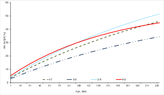
Figure 1 Growth curves for Katahdin (KT), Blackbelly (BB), Dorper (DR) and Rambouillet (RB) sheep breeds based on Brody model 

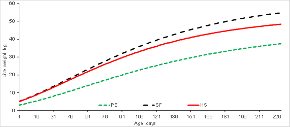
Figure 2: Growth curves for Pelibuey (PE), Suffolk (SF) and Hampshire (HS) sheep breeds based on von Bertalanffy model 

Other studies highlight how different NLM provide the best fit for different sheep breeds. Similar studies with the Baluchi⁵, Hemsin¹⁷, and West African Dwarf¹⁸ sheep breeds reported that the BRO model was best fitted to describe growth. In an analysis of growth in Morada Nova sheep⁴, the Meloun I and Meloun III models were found to have the best fit, with growth patterns similar to those in the BRO and MIT models used in the present study. However, in the Segureñas⁹ and Awassi breeds¹⁹ the VBE model has been found to have the best fit.

Marked differences were observed in AW in the seven evaluated breeds (Table 4). This parameter tended to be highest in the BRO and MIT models, and lowest in the LOG and VER models. Average values were 44.6 kg in BB, 49.2 kg in RB, 52.9 kg in PE, 55.6 kg in HS, 60.2 kg in KT, 64.7 in SF and 65.2 in DR. Increases in female AW affect maintenance, reproduction and waste value needs. Given that a large percentage of lamb production costs occur in ewes, increasing ewe size can raise production costs; however, asymptotic weight can be kept constant in selection programs while GR is maximized^14,20. Since GR refers to the velocity of growth relative to AW, high GR can result in AW being attained at a younger age. Growth rate (GR) is financially important because it can be used to determine the optimal moment for slaughter, which is usually when the animal has reached maximum GR^13,21.

The correlations between AW and GR are essential in strategies aimed at modifying growth curves^15,21. All correlations between AW and GR in the present study were negative and high (-0.70 to -0.99). These negative correlations suggest certain growth curve characteristics: a) older AWs do not derive from high GRs; b) a lower GR may lengthen the time to reach AW; and c) in genetic improvement schemes, GR can be increased without affecting AW^7,15,22.

Conclusions and implications

For the Hampshire, Pelibuey and Suffolk breeds, a nonlinear model based on the von Bertalanffy model produced sigmoid type growth curves with an inflection point at 40 to 57 d. For the Katahdin, Blackbelly, Dorper and Rambouillet breeds, a nonlinear model based on the Brody model resulted in growth curves with a continuous growth rate and no inflection point. The differences observed between the breeds as manifested in curve pattern and growth indicators express varying genetic potential, which can be exploited in different production systems.

REFERENCES

1. CONARGEN. Guía técnica de programas de control de producción y mejoramiento genético en ovinos. Consejo Nacional de los Recursos Genéticos Pecuarios. México, DF. 2010. [ Links ]
2. Lewis RM, Emmans GC, Dingwall WS, Simm G. A description of the growth of sheep and its genetic analysis. Anim Sci 2002;74:51-62. [ Links ]
3. Agudelo GDA, Cerón MF, Restrepo LFB. Modelación de las funciones de crecimiento aplicadas a la producción animal. Rev Colomb Cienc Pecu 2008;21:39-58. [ Links ]
4. de Andrade SL, Souza PLC, Mendes CHM, Fonseca S, Gomes da SF. Traditional and alternative nonlinear models for estimating the growth of Morada Nova sheep. Rev Bras Zootec 2013;42:651-655. [ Links ]
5. Bahreini BMR, Aslaminejad AA, Sharifi AR, Simianer H. Comparison of mathematical models for describing the growth of Baluchi sheep. J Agr Sci Tech 2014;14:57-68. [ Links ]
6. Teixeira NMR, da Cruz JF, Neves FH, Santos SE, Souza CPL, Mendes MC. Descrição do crescimento de ovinos Santa Inês utilizando modelos não-lineares seleccionados por análise multivariada. Rev Bras Saude Prod Anim 2016;17:26-36. [ Links ]
7. Malhado CHM, Carneiro PL, Alfonso PRA, Souza AA, Sarmento JLR. Growth curves in Dorper sheep crossed with the local Brazilian breeds, Morada Nova, Rabo Largo, and Santa Inês. Small Ruminant Res 2009;84:16-21. [ Links ]
8. Ben HM, Atti N. Comparison of growth curves of lamb fat tail measurements and their relationship with body weight in Babarine sheep. Small Ruminant Res 2013;95:120-127. [ Links ]
9. Lupi TM, Nogales S, León JM, Barba C, Delgado JV. Characterization of commercial and biological growth curves in the Segureña sheep breed. Animal 2015;9:1341-1348. [ Links ]
10. SAS. SAS/STAT User's Guide (Release 9.0). Cary NC, USA: SAS Inst. Inc. 2005. [ Links ]
11. Motulsky H, Christopoulos A. Fitting models to biological data using linear and nonlinear regression. A practical guide to curve fitting. Graph Pad Software Inc. 2003. [ Links ]
12. Hossein-Zadeh NG. Modeling the growth curve of Iranian Shall sheep using non-linear growth models. Small Ruminant Res 2015;130:60-66. [ Links ]
13. Hossein-Zadeh NG, Golshani M. Comparison of non-linear models to describe growth of Iranian Guilan sheep. Rev Colomb Cienc Pecu 2016;29:199-209. [ Links ]
14. Owens FN, Dubeski P, Hanson CF. Factors that alter the growth and development of ruminants. J Anim Sci 1993;71:3138-3150. [ Links ]
15. Lupi TM, León JM, Nogales S, Barba C, Delgado JV. Genetic parameters of traits associated with the growth curve in Segureña sheep. Animal 2016;9:729-735. [ Links ]
16. Ribeiro de FA. Curvas de crescimento na produçã animal. Rev Bras Zootec 2005;34:786-795. [ Links ]
17. Kopuzlu S, Sezgin E, Esenbuga E, Bilgin OC. Estimation of growth curve characteristics of Hemsin male and female sheep. J Appl Anim Res 2014;42:228-232. [ Links ]
18. Gbangboche AB, Glele-Kakai R, Salifou S, Albuquerque LG, Leroy PL. Comparison of nonlinear growth models to describe the growth curve in West African Dwarf sheep. Animal 2008;2:1003-1012. [ Links ]
19. Topal M, Ozdemir M, Aksakal V, Yildiz N, Dogru U. Determination of the best nonlinear function in order to estimate growth in Morkaraman and Awassi lambs. Small Ruminant Res 2004;55:229-232. [ Links ]
20. Bathaei SS, Leroy PL. Growth and mature weight of Mehraban Iranian fat-tailed sheep. Small Ruminant Res 1996;22:155-162. [ Links ]
21. Lambe NR, Navajas EA, Simm G, Bünger L. A genetic investigation of various growth models to describe growth of lamb of two contrasting breeds. J Anim Sci 2006;84:2642-2654. [ Links ]
22. Acioli da SLS, Bossi FA, de Lima da SF, Mendes GB, de Oliveira SR, Tonhati H, da Costa BC. Growth curve in Santa Inês sheep. Small Ruminant Res 2012;105:182-185. [ Links ]
Received: March 10, 2018; Accepted: September 27, 2018
Este es un artículo publicado en acceso abierto bajo una licencia
Creative Commons