


Servicios Personalizados
Revista
Articulo
 texto en
  Inglés (pdf)
 Artículo en XML
 Referencias del artículo
 Enviar artículo por email
Indicadores
-
 Citado por SciELO
 -
 Accesos
Links relacionados
-
 Similares en
SciELO
Similares en
SciELO
Compartir

 Permalink
Revista mexicana de ciencias agrícolas
versión impresa ISSN 2007-0934
Rev. Mex. Cienc. Agríc vol.12 no.8 Texcoco nov./dic. 2021 Epub 02-Mayo-2022
https://doi.org/10.29312/remexca.v12i8.2267
Articles
Yield and stability of soybean genotypes for the tropics of Mexico
1Campo Experimental Las Huastecas-INIFAP. Carretera Tampico-Mante km 55, Villa Cuauhtémoc, Tamaulipas, México. CP. 89610. (maldonado.nicolas@inifap.gob.mx; ascencio.guillermo@inifap.gob.mx; garcia.juliocesar@inifap.gob.mx).
Currently, climate change forces plant breeders to develop genotypes adapted to mega-environments, which guarantees the correct production of the crop. The objective of this study was to determine the potential in grain yield and stability of soybean genotypes. For these purposes, 15 soybean genotypes (seven varieties and eight experimental lines) were evaluated over four years (2014, 2015, 2016 and 2017), in a 5x5 square lattice design with three repetitions. The analysis of variance revealed significant differences in years, genotypes, and in the genotype-by-year interaction. Being the source of variation years, the one that had the greatest impact on yield with 84.3%, followed by the genotype-by-year interaction (10%) and genotypes (5.6%). Likewise, the conditions of 2014 were more conducive for genotypes to have a higher yield. Regarding genotypes, G15, G7, G5 and G2 had the highest yield values throughout the four years. In terms of stability and yield, the relative yield method and the GGE Biplot representation agreed that the genotypes that have these two characteristics are G7 and G2. On the other hand, two mega-environments formed, being genotype G15 the winner with respect to its performance in the first mega-environment, where the years 2015, 2016 and 2017 were included, in the same way, genotype G5 was the winner in the second mega-environment constituted by the year 2014. The two methods when complementing each other mostly explained the phenotypic variation in yield.
Keywords: biplot; ideal genotype; relative yield
Actualmente el cambio climático obliga a los fitomejoradores a desarrollar genotipos adaptados a mega-ambientes, lo que garantiza la correcta producción del cultivo. El objetivo de este estudio fue determinar el potencial en rendimiento de grano y estabilidad de genotipos de soya. Para estos fines, se evaluaron 15 genotipos de soya (siete variedades y ocho líneas experimentales) a través de cuatro años (2014, 2015, 2016 y 2017), en un diseño látice cuadrado 5x5 con tres repeticiones. El análisis de varianza reveló diferencias significativas en años, genotipos y en la interacción genotipos por años. Siendo la fuente de variación años, la que tuvo mayor impacto en el rendimiento con un 84.3%, seguido de la interacción genotipos por años (10%) y de genotipos (5.6%). Asimismo, las condiciones del 2014 fueron más propicias para que los genotipos tuvieran un mayor rendimiento. Con relación a los genotipos, el G15, G7, G5 y G2 presentaron los mayores valores de rendimiento a través de los cuatro años. En cuanto a estabilidad y rendimiento el método de rendimiento relativo y la representación Biplot GGE coincidieron en que los genotipos que poseen estas dos características son G7 y G2. Por otro lado, se formaron dos mega-ambientes siendo el genotipo G15 el ganador respecto a su desempeño en el primer mega-ambiente donde estuvieron incluidos los años 2015, 2016 y 2017, de la misma forma el genotipo G5 fue el ganador en el segundo mega-ambiente constituido por el año 2014. Los dos métodos al complementarse explicaron mayormente la variación fenotípica del rendimiento.
Palabras clave: biplot; genotipo ideal; rendimiento relativo
Introduction
Soybean [Glycine max (L.) Merrill] is one of the most important crops in the world due to its diversity of uses and currently, the main source of edible oil among oilseed crops (Bhartiya et al., 2014). It can adapt to various climates, although it develops optimally in tropical regions (Pecina et al., 2005). It is grown mainly in North America, South America and Asia; however, the main exporting countries are the United States and Brazil (Kumudini, 2010). According to the growing demand for the crop, superior genotypes that have yield potential and stability are sought, for which tests are used in several years and localities (Lu’quez et al., 2002; Smith et al., 2005; Yang et al., 2009).
In this regard, one of the main challenges faced by plant breeders is the differential response of genotypes as a function of the environment (Kang and Gorman, 1989), known as genotype-by-environment interaction (GEI). The expression of each characteristic in a crop is the result of the effect of genotype (G), the effect of the environment (E) and GEI (Yan and Tinker, 2005). But genotypic evaluation is limited only to the main effects of G, while GEI is ignored without considering the stability of genotypes (Yan and Tinker, 2006; Bhartiya et al., 2017).
GEI using multi-environment trials (MET) makes it possible to accurately evaluate crop yields in different environments, predict yield levels, and examine genotype stability for the selection of the best genotypes in improvement programs (Magari and Kang, 1993; Ebdon and Gauch, 2002; Mustapha and Bakari, 2014). A wide range of statistical techniques have been developed to study GEI, including univariate models, such as regression slope, deviation from the regression, environmental variance and yield stability, and multivariate models, such as the genotype main effect plus genotype by environment (GGE) and additive main effects and multiplicative interaction (AMMI) (Finlay and Wilkinson, 1963; Eberhart and Russell, 1966; Kang, 1993; Yan, 2001).
These last two models are based on the principal component (PC) analysis and have the ability to classify genotypes based on some characteristic of interest and the stability that this characteristic shows in each genotype when evaluating them in different environments (Casanoves et al., 2005). For research purposes and to delineate mega-environments, the AMMI model, the SREG model and SHMM are considered equally effective (Gauch et al., 2008). The present research was carried out with the aim of comparing the relative yield method and the GGE Biplot representation and identifying soybean genotypes with good yield and stability under rainfed conditions in the southern region of Tamaulipas, Mexico.
Materials and methods
Location of the experimental site
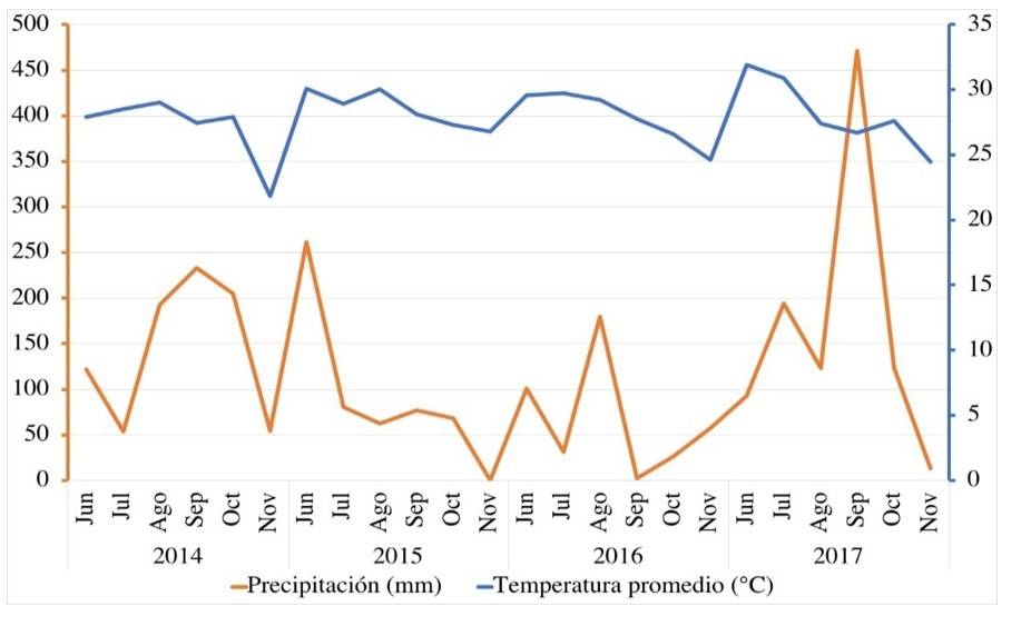
The research was carried out in the spring-summer (P-V) cycles from 2014 to 2017, under rainfed conditions at the National Institute of Forestry, Agricultural and Livestock Research (INIFAP, for its acronym in Spanish), Las Huastecas Experimental Field, located at 22º 33’ 57.88” north latitude and 98º 09’ 52.47” west longitude with an altitude of 17 m. This region has a semi-warm humid tropical climate, with an average annual temperature of 24.5 ºC and a rainfall of 842 mm.
Plant material
Fifteen genotypes were used, including varieties and experimental lines from the soybean genetic improvement area of the INIFAP Annual Oilseeds Program, which have different characteristics of agronomic interest such as health, appearance, grain production and adaptability to the Huasteca region (Table 1).
Methodology
The preparation of the land was carried out starting with the fallow at a depth of 30 cm, followed by two passes of harrow at 20 days after the fallow and finally the furrowing was carried out at a distance of 76 cm.
Sowing was carried out on plots of 4 furrows of 5 m in length with a density of 250 000 plants ha-1. The rest of the agronomic management was carried out according to the soybean technological package for southern Tamaulipas (Maldonado, 2017). At the time of harvest, the grain yield was recorded with a moisture content of 14% in units of kg ha-1.
Design
The experiment was established under a 5x5 square lattice design, with three repetitions. Two factors were considered, the first was the genotypes, which were randomized in the lattice, and the second the years.
Statistical analysis
With the information from each environment, the combined analysis of variance was performed, and the Tukey test was applied with 0.05 of significance level for the comparison of the means of yields of the genotypes and years. To estimate yield stability, the relative yield (RY) method was used, this method consists of expressing the yield of each genotype in each environment in a relative way to the average of the given environment, assigning the latter the value of 100. Genetic materials that have a yield lower than the average of all genotypes in the same environment will have RY values of less than 100, while those with higher yields will have values greater than 100.
The standard deviation, calculated as the square root of the variance of the relative yields of each genetic material across environments, is the measure of stability. The most stable genotypes will be those with the lowest standard deviation (Yau and Hamblin, 1994). A line graph was developed for the interpretation of climate data. For the genotype-by-environment interaction, principal component analyses were performed, from which GGE Biplot graphs (genotype plus genotype by environment) were developed (Yan et al., 2007). Analyses were carried out using the R statistical package version 3.6 (R, 2020) and SAS version 9.4 (SAS, 2014).
Results and discussion
Analysis of variance
In the present work, it was observed that the repetitions within years did not influence yield so it can be assumed that the land conditions were homogeneous. On the other hand, years, as well as genotypes and their interaction, in addition to the first two main components, showed significant differences (p≤ 0.01), this could be due to the genetic diversity presented by the genotypes, the particular conditions that the years presented and the different response of the genotypes in each year.
Regarding heritability, this character showed low values, where the environmental component contributed the largest proportion of the total variation, so it is assumed that the character is controlled by several genes of small effect (Table 2). Likewise, the relative contribution of the variance of the genotype-by-year component was higher compared to the component of genotype variance. These results are similar to those reported by Shukla et al. (2015); Vaezi et al. (2017), who mention that most of the variation is attributable to environmental effects followed by the genotype-by-environment interaction and genotype.
Table 2 Principal components and mean squares of the analysis of variance for the yield variable.
| SV | DF | MS | SS(%) | |
| Years | 3 | 22 496734 | ** | 74.7 |
| Rep (years) | 8 | 99 660 | ns | 0.9 |
| Gen | 14 | 322 278 | ** | 5 |
| Gen*years | 42 | 191 069 | ** | 8.9 |
| CP1 | 16 | 248 131 | ** | |
| CP2 | 14 | 202 728.5 | ** | |
| CP3 | 12 | 96 615.4 | ns | |
| Error | 112 | 84 894 | 10.5 | |
| H2 (%) | 8 | |||
| R2 (%) | 89 | |||
| CV (%) | 11.2 |
*= significant at 0.05; **= significant at 0.01; ns= not significant; SV= source of variation; DF= degrees of freedom; Rep= repetition; Gen= genotypes; CP= principal components; R2= coefficient of determination; CV= coefficient of variation; MS= mean squares; SS(%)= percentage of sum of squares.
Comparison of means and stability
According to Table 3, a variation was observed in overall yield averages. As for the years, on average 2014 had the highest yield value, being 32.6% higher than the average of the rest of the years. Likewise, 2016 obtained the lowest value, this was related to the rainfall that occurred during the crop cycle, and especially the amount and distribution of rainfall that occurred during the grain-filling period. This coincides with López-Castañeda (2011), who mentions that water stress reduces stomatal conductance and net assimilation rate during grain filling, which reduces yield.
Table 3 Relative yield of soybean genotypes over four years.
| Gen | 2014 | 2015 | 2016 | 2017 | Average yield | RY | s² | |||||||
| Yield | (%) R | Yield | (%) R | Yield | (%) R | Yield | (%) R | |||||||
| G15 | 3 613.8 | 106 | 3 118 | 134 | 1 878.3 | 108 | 3 458.2 | 123 | 3 017.1 a | 118 | 13 | |||
| G7 | 3 500.4 | 103 | 2 785.4 | 119 | 1 784.7 | 103 | 3 000.8 | 107 | 2 767.8 ab | 108 | 7.8 | |||
| G5 | 3 908.7 | 115 | 2 237.2 | 96 | 1 903.5 | 110 | 2 842 | 101 | 2722.9 abc | 106 | 8.5 | |||
| G2 | 3 464.6 | 102 | 2 358.8 | 101 | 1 705.6 | 98 | 2 962.1 | 106 | 2622.8 abc | 102 | 2.9 | |||
| G14 | 3 518.8 | 104 | 2 322.1 | 100 | 1 950.2 | 113 | 2 617 | 93 | 2 602 bc | 102 | 8.1 | |||
| G9 | 3 798.6 | 112 | 2 011.1 | 86 | 1 670 | 96 | 2 833.2 | 101 | 2 578.2 bc | 99 | 10.6 | |||
| G3 | 3 636.1 | 107 | 2 337.1 | 100 | 1 559.6 | 90 | 2 752.7 | 98 | 2 571.4 bc | 99 | 7 | |||
| G1 | 3 095.1 | 91 | 2 514.9 | 108 | 1 742.5 | 101 | 2 906.8 | 104 | 2 564.8 bc | 101 | 7.1 | |||
| G13 | 3 124.6 | 92 | 2 450.5 | 105 | 1 723.6 | 99 | 2 905.3 | 103 | 2 551 bc | 100 | 5.9 | |||
| G10 | 2 903.1 | 85 | 1 912.9 | 82 | 2 281 | 132 | 2 956.2 | 105 | 2 513.3 bc | 101 | 22.8 | |||
| G6 | 3 179.3 | 94 | 2 270.9 | 97 | 1 567.8 | 90 | 2 801.7 | 100 | 2 454.9 bc | 95 | 4.1 | |||
| G8 | 3 525.3 | 104 | 2 349.8 | 101 | 1 530.5 | 88 | 2 368.7 | 84 | 2 443.6 bc | 94 | 9.4 | |||
| G11 | 3 010.5 | 89 | 2 385.7 | 102 | 1 753 | 101 | 2 412.3 | 86 | 2 390.4 bc | 94 | 8.4 | |||
| G4 | 3 419.9 | 101 | 1 835.2 | 79 | 1 530.3 | 88 | 2 706.4 | 96 | 2 373.0 bc | 91 | 9.7 | |||
| G12 | 3 280 | 97 | 2 080.7 | 89 | 1 419.8 | 82 | 2 585.9 | 92 | 2 341.6 c | 90 | 6.1 | |||
| x | 3398.6 a | 100 | 2331.4 c | 100 | 1733.4 d | 100 | 2807.3 b | 100 | ||||||
Soybean genotypes with the same letter are statistically the same; Gen= genotypes; R(%)= relative percentage; ͞x= average; RY= relative yield; s²= standard deviation of relative yield.
On the other hand, temperature was not a limiting factor since it decreased considerably when reaching the stage of physiological maturity (R8) (Figure 1). The genotypes that stood out in terms of their yield were G15 (Tamesí), G7 (H98-1325), G5 (H10-3056) and G2 (H02-1987), surpassing the average of the rest of the genotypes by 17.5, 10, 8.6 and 5.1% respectively. These percentages in terms of years and genotypes confirm the impact that the environment has on the expression of the character. Regarding the RY method, the genotypes that had the highest relative yield and stability were G7 (H98-1325), G5 (H10-3056) and G2 (H02-1987), having values higher than 100 in RY and a lower standard deviation compared to the average.
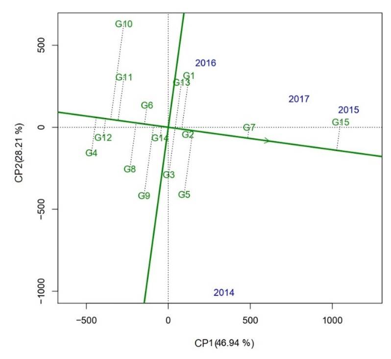
Regarding principal components (CP) for yield, the first two CPs explained 75.15% of the total variation. CP1 explained the largest variation (46.94%) followed by CP2 (28.21%). To represent stability in this biplot, the axis of the environment coordinate (AEC) abscissa is the green horizontal line of a single arrow passing through the origin of the biplot. With respect to the axis of the AEC ordinate, it is represented with the green vertical line that passes through the biplot origin and is perpendicular to the AEC abscissa, in this way, the genotypes that show greater distance on the AEC abscissa in any direction will be more unstable (Yan et al., 2007).
Therefore, genotype G2 (H02-1987), followed by G14 (Huasteca 700) and G7 (H98-1325) were the most stable, while genotypes G10 (Huasteca 200), G9 (Huasteca 100) and G5 (H10-3056) were highly unstable in all years for the yield variable (Figure 2). In this sense, Brar et al. (2010) mentions that the ideal genotype must have high stability to ensure adaptability to a target region and minimize the risk of yield loss due to environmental conditions.
Ideal genotype
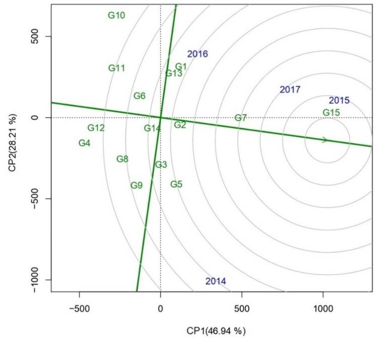
In this aspect, the four genotypes that came closest to the ideal were G15 (Tamesí), having the highest average yield, followed by G7 (H98-1325), G5 (H10-3056) and G2 (H02-1987). On the other hand, genotypes G3 (H02-2082), G13 (Huasteca 600) and G14 (Huasteca700) had a behavior similar to the general average. However, G4 (H10-0556), G12 (Huasteca 400) and G11 (Huasteca 300) were considered the least ideal as they had on average the lowest yield over the years.
Genotype G10 is also on this last list because it had the most extreme values (high and low) over the years (Figure 3). These observations relate to Farshadfar et al. (2013), who mention that an ideal genotype is one that has a high average grain yield and high stability. It should be noted that the genotypes were distributed in the four quadrants, which indicates the genetic diversity that they have, which is indispensable in a genetic improvement program (Figure 3). Rimieri (2017) mentions that the variability available for selection is found in previously adapted genotypes, since the variability of species in the wild generally cannot be used directly.
Mega-environments
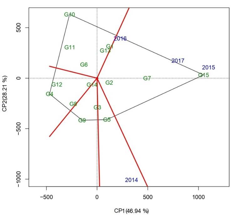
The relationship shown by the years depended on the cosine of the angle of the vectors, which approximates the correlation coefficient, where the acute angle indicated a positive relationship, however the obtuse angle revealed a negative relationship and the right angles meant that there was none (Yan, 2002; Haider et al., 2017), being able to form two groups of mega-environments: the first group was formed by the years 2015, 2016 and 2017, likewise, the second group was formed by the year 2014. The latter presented a right to obtuse angle with respect to the years of the first group. On the other hand, the years 2014 and 2015 were the most discriminatory due to the length of their vectors, which were greater than the rest of the years. This data is essential to reduce costs and improve the accuracy of selection (Imtiaz et al., 2013).
In order to observe the best genotypes in each environment and groups of environments, the ‘which-won-where’ pattern was used. The biplot was divided into five sectors, where the four years fell in two, indicating the presence of significant cross interaction. According to Yan et al. (2007), when different environments fall in different sectors, it implies that there are high-yield genotypes for those sectors. Likewise, Yan and Kang (2003) mention that from the polygonal view, the presence or absence of the genotype-by-environment cross-interaction that explains the existence of different mega-environments can be better observed.
On the other hand, genotype G15 (Tamesí) had a high yield in the years 2015, 2016 and 2017, while genotype G5 (H10-3056) showed the best yield in 2014, suggesting that specialized genotypes can be developed for specific environments (Figure 4). This behavior is because the genotypes located at the vertices of each sector indicated a better or worse behavior in one or another environment (Yan et al., 2000; Dia et al., 2016).
According to the above results, genotypes could be classified into four groups. The first group was made up of genotypes G15 (Tamesí), G7 (H98-1325) and G2 (H02-1987), these being the most yielding and stable, which are the main characteristics for improvement. The second was made up of genotypes G1 (H02-1337), G13 (Huasteca 600) and G5 (H10-3056), which were yielding but unstable, ideal for crossbreeding and selection.
The third group consisted of genotypes G12 (Huasteca 400), G4 (H10-0556), G6 (H98-1240) and G14 (Huasteca 700), stable but with yield equal to or less than the average. Finally, the fourth group was formed by genotypes G11 (Huasteca 300), G9 (Huasteca 100), G8 (H98-1521), G3 (H02-2082) and G10 (Huasteca 200), unstable with yield equal to or less than the average, these last two groups would be discarded for a genetic improvement program. Related to this, López et al. (2011) mention that studies of adaptability and stability of yield are of vital importance to determine the response of genotypes in different localities, years and cycles of the crop.
Conclusions
The RY method and the GGE Biplot representation turned out to be efficient when complementing each other, since on the one hand the first one considers the genotypes and part of the environment; however, in the second, the genotype effect plus its interaction with the environment is determined. Genotypes G15, G7 and G2 will contribute with greater yield potential per unit area and good stability for the tropics of Mexico.
Literatura citada
Bhartiya, A.; Aditya, J. P.; Kumari, V.; Kishore, N.; Purwar, J. P.; Agrawal, A. and Kant, L. 2017. GGE biplot & AMMI analysis of yield stability in multi-environment trial of soybean[Glycine max (L.) Merrill] genotypes under rainfed condition of north western Himalayan hills. J. Anim. Plant Sci. 27(1):227-238. [ Links ]
Bhartiya, A.; Singh, K.; Aditya, J. P.; Puspendra and Gupta, M. 2014. Residual relative heterosis and heterobeltiosis for different agro morphological traits as selection index in early segregating generation of soybean [Glycine max (L.) Merrill] crosses. Soybean res. 12(1):28-35. [ Links ]
Brar, K. S.; Singh, P.; Mittal, V. P.; Singh, P.; Jakhar, M. L.; Yadav, Y.; Sharma, M. M.; Shekhawat, U. S. and Kumar, C. 2010. GGE biplot analysis for visualization of mean performance and stability for seed yield in taramira at diverse locations in India. J. Oilseed Brassica. 1(2):66-74. [ Links ]
Casanoves, F.; Baldessari, J. and Balzarini, M. 2005. Evaluation of multienvironment trials of peanut cultivars. Crop Sci. 45(1):18-26. doi:10.2135/cropsci2005.0018. [ Links ]
Dia, M.; Wehner, T. C.; Hassell, R.; Price, D. S.; Boyhan, G. E.; Olson, S.; King, S.; Davis, A. R. and Tolla, G. E. 2016. Genotype environment interaction and stability analysis for watermelon fruit yield in the United States. Crop Sci. 56(4):1645-1661. doi:10.2135/ cropsci2015.10.0625. [ Links ]
Ebdon, J. S. and Gauch, H. G. 2002. Additive main effect and multiplicative interaction analysis of national turfgrass performance trials. Crop Sci. 42(2):497-506. doi:10.2135/cropsci200 2.0489. [ Links ]
Eberhart, S. T. and Russell, W. A. 1966. Stability parameters for comparing varieties. Crop Sci. 6(1):36-40. doi: 10.2135/cropsci196 6.0011183X000600010011x. [ Links ]
Farshadfar, E.; Rashidi, M.; Jowkar, M. M. and Zali, H. 2013. GGE Biplot analysis of genotype environment interaction in chickpea genotypes. Eur. J. Exp. Biol. 3(1):417-423. [ Links ]
Finlay, K. W. and Wilkinson, G. N. 1963. The analysis of adaptation in a plant breeding programme. Aust. J. Agric. Res. 14(6):742-754. doi: 10.1071/AR9630742. [ Links ]
Gauch, H. G.; Piepho, H. P. and Annicchiarico, P. 2008. Statistical analysis of yield trials by AMMI and GGE: Further considerations. Crop Sci. 48(3):866-889. doi:10.2135/cropsci2007. 09.0513. [ Links ]
Haider, Z.; Akhter, M.; Mahmood, A. and Khan, R. A. R. 2017. Comparison of GGE biplot and AMMI analysis of multi-environment trial (MET) data to assess adaptability and stability of rice genotypes. African J. Agric. Res. 12(51):3542-3548. doi:10.5897/AJAR2017.12528. [ Links ]
Imtiaz, M.; Malhotra, R. S.; Singh, M. and Arslan, S. 2013. Identifying high yielding, stable chickpea genotypes for spring sowing: specific adaptation to locations and sowing seasons in the Mediterranean region. Crop Sci. 53(4):1472-1480. doi:10.2135/cropsci2012.10.0589. [ Links ]
Kang, M. S. 1993. Simultaneous selection for yield and stability in crop performance trials: Consequences for growers. Agron. J. 85(3):754-757. [ Links ]
Kang, M. S. and Gorman, D. P. 1989. Genotype × environment interaction in maize. Agron. J. 81(4):662-664. doi: 10.2134/agron j1989.00021962008100040020x. [ Links ]
Kumudini, S. 2010. Soybean growth and development. The soybean: botany, production and uses. (Ed.) by Guriq Singh. Ludhiana, India. 23 p. [ Links ]
López-Castañeda, C. 2011. Variación en rendimiento de grano, biomasa y número de granos en cebada bajo tres condiciones de humedad del suelo. Trop. Subtrop. Agroecosyst. 14(3):907-918. [ Links ]
López, S. E.; Acosta, G. J. A.; Tosquy, V. O. H.; Salinas, P. R. A.; Sánchez, G. B. M.; Rosales, S. R.; González, R. C.; Moreno, G. T.; Villar, S. B. Cortinas; E. H. M. y Zandate, H. R. 2011. Estabilidad de rendimiento en genotipos mesoamericanos de frijol de grano en México. Rev. Mex. Cienc. Agríc. 2(1):29-40. [ Links ]
Lu’quez, J. E.; Aguirreza’bal, L. A. N.; Aguero, M. E. and Pereyra, V. R. 2002. Stability and adaptability of cultivars in non- balanced yield trials: comparison of methods for selecting ‘high oleic’ sunflower hybrids for grain yield and quality. J. Agron. Crop Sci. 188(4):225-234. doi:10.1046/j.1439-037X.2002.00562.x. [ Links ]
Magari, R. and Kang, M. S. 1993. Genotype selection via a new yield stability statistic in maize yield trials. Euphytica. 70(1-2):105-111. doi: 10.1007/BF00029647. [ Links ]
Maldonado, M. N. 2017. Soya de temporal y riego para el sur de Tamaulipas ciclo P-V. Agenda Técnica Agrícola Tamaulipas. Instituto Nacional de Investigaciones Forestales, Agrícolas y Pecuarias (INIFAP). Ciudad de México. 92-105 pp. [ Links ]
Mustapha, M. and Bakari, H. R. 2014. Statistical evaluation of genotype by environment interactions for grain yield in millet (Penniisetum glaucum (L.) R. Br.). Int. J. Eng. Sci. 3(9):7-16. [ Links ]
Pecina, Q. V.; Maldonado, H. L.; Maldonado, M. N.; Simpson, J.; Martínez, V. O. y Gil, V. K. C. 2005. Diversidad genética en soya del Trópico Húmedo de México determinada con marcadores AFLP. Rev. Fitotec. Mex. 28(1):63-69. [ Links ]
R. 2020. R: A Language and environment for statistical computing. R foundation for statistical computing. Vienna, Austria. Retrieved from http://www.r-project.org/. [ Links ]
Rimieri, P. 2017. La diversidad y la variabilidad genéticas: dos conceptos diferentes asociados al germoplasma y al mejoramiento genético vegetal. BAG. J. Basic Appl. Gen. 28(2):7-13. [ Links ]
SAS. 2014. SAS: Business analytics and business intelligence software. NC, USA: SAS Inst. Retrieved from http://www.sas.com/en-us/home.html. [ Links ]
Shukla, S.; Mishra, B. K.; Mishra, R.; Siddiqui, A.; Pandey, R. and Rastogi, A. 2015. Comparative study for stability and adaptability through different models in developed high thebaine lines of opium poppy (Papaver somniferum L.). Ind. Crops prod. 74:875-886. doi:10.1016/j.indcrop.2015.05.076. [ Links ]
Smith, A. B.; Cullis, B. R. and Thompson, R. 2005. The analysis of crop cultivar breeding and evaluation trials: An overview of current mixed model approaches. J. Agric. Sci. 143(06):449-462. doi: 10.1017/S0021859605005587. [ Links ]
Vaezi, B.; Pour-Aboughadareh, A.; Mohammadi, R.; Armion, M.; Mehraban, A.; Hossein-Pour, T. and Dorii, M. 2017. GGE biplot and AMMI analysis of barley yield performance in Iran. Cereal res. Commun. 45(3):500-511. doi:10.1556/0806.45.2017.019. [ Links ]
Yan, W. 2001. GGE biplot a Windows application for graphical analysis of multienvironment trial data and other types of two-way data. Agron. J. 93(5):1111-1118. [ Links ]
Yan, W. and Tinker, N. A. 2005. An integrated biplot analysis system for displaying, interpreting and exploring genotype environment interaction. Crop Sci. 45(3):1004-1016. doi:10.2135/cropsci2004.0076. [ Links ]
Yan, W. and Kang, M. S. 2003. GGE biplot analysis: a graphical tool for breeders, geneticists, and agronomists. CRC Press. Boca Raton, London, New York, Washington, D.C. retrieved from https://content.taylorfrancis.com/books/download?dac=c2009-0-09571-8&isbn=978 0429122729&format=googlepreviewpdf. 263 p. [ Links ]
Yan, W. 2002. Singular-value partitioning in biplot analysis of multienvironment trial data. Agron. J. 94(5):990-996. doi:10.2134/AGRONJ2002.9900. [ Links ]
Yan, W.; Hunt, L. A.; Sheng, Q. and Szlavnics, Z. 2000. Cultivar evaluation and mega-environment investigation based on the GGE biplot. Crop Sci. 40(3):597-605. doi:10.2135/cropsci2000. 403597x. [ Links ]
Yan, W.; Kang, M. S.; Ma, B.; Woods, S. and Cornelius, P. L. 2007. GGE biplot vs. AMMI analysis of genotype-by-environment data. Crop sci. 47(2):643-655. doi:10.2135/cropsci2006. 06.0374. [ Links ]
Yan, W. and Tinker, N. A. 2006. Biplot analysis of multi-environment trial data: principles and applications. Can. J. Plant Sci. 86(3):623-645. doi:10.4141/P05-169. [ Links ]
Yang, R. C.; Crossa, J.; Cornelius, P. L. and Burgueño, J. 2009. Biplot analysis of genotype environment interaction: proceed with caution. Crop Sci. 49(5):1564-1576. doi:10.2135/cropsci2008.11.0665. [ Links ]
Yau, S. K. and Hamblin, J. 1994. Relative yield as a measure of entry performance in variable environments. Crop Sci. 34(3):813-817. doi:10.2135/cropsci1994.0011183X0034000 30038x. [ Links ]
Received: July 01, 2021; Accepted: September 01, 2021
 Este es un artículo publicado en acceso abierto bajo una licencia Creative Commons
