


Serviços Personalizados
Journal
Artigo
 texto em
  Inglês (pdf)
 Artigo em XML
 Referências do artigo
 Enviar este artigo por email
Indicadores
-
 Citado por SciELO
 -
 Acessos
Links relacionados
-
 Similares em
SciELO
Similares em
SciELO
Compartilhar

 Permalink
Revista mexicana de ciencias agrícolas
versão impressa ISSN 2007-0934
Rev. Mex. Cienc. Agríc vol.11 no.8 Texcoco Nov./Dez. 2020 Epub 13-Dez-2021
https://doi.org/10.29312/remexca.v11i8.2747
Articles
Prediction of water erosion in the Sumidero Canyon basin, Chiapas
1Manejo Integral de Cuencas SA de CV. José María Pino Súarez Mz. 15, Lt. 19, Nezahualcóyotl, Texcoco, Estado de México. CP. 56263. Tel. 595 9529824. (elibeth.tb@gmail.com; jcortesbecerra@gmail.com; ltorres-cedillo@hotmail.com; pedro-riverat@hotmail.com).
2Campo Experimental Bajío-INIFAP. Carretera San Miguel de Allende-Celaya km 6.5, Celaya, Guanajuato. CP. 38110.
In the Sumidero Canyon Basin, Chiapas state, Mexico, the soil is a component of the natural environment strongly affected by erosion due to inadequate management of the soil resource. Measuring soil erosion is time consuming and data on soil erosion rates in Mexico are limited and punctual and provide little information on soil loss rates at the basin level. In the present study, methodologies were used for the application of the USLE/RUSLE, developed in various studies and countries, in order to carry out the cartography of water erosion of the Sumidero Canyon Basin, which constitutes a significant tool for making decisions. in the management and conservation of soils. A series of methodological tools is proposed for the generation of the water erosion cartography using information in Mexico at various scales. The results are presented as an average annual geographic reference of soil loss and its monthly distribution. The analysis of results indicates that 73% of the basin presents some degree of erosion, that June is the month that erosion is greatest (7 021 906.9 t) and that the average annual erosion in the study area is 41.5 t ha-1 year-1.
Keywords: GIS; natural resources; RUSLE; USLE
En la cuenca del Cañón del Sumidero, estado de Chiapas, México, el suelo es un componente del medio natural fuertemente afectado por la erosión debido al manejo inadecuado del recurso suelo. La medición de la erosión del suelo lleva mucho tiempo y los datos de las tasas de erosión del suelo en México son limitados y puntuales, además, aportan poca información sobre las tasas de pérdida de suelo a nivel de cuenca. En el presente estudio se usaron metodologías para la aplicación de la USLE/RUSLE, desarrolladas en diversos estudios y países, con el propósito de realizar la cartografía de erosión hídrica de la cuenca del Cañón del Sumidero, la cual constituye una herramienta significativa para tomar decisiones en el manejo y conservación de suelos. Se propone una serie de herramientas metodológicas para la generación de la cartografía de erosión hídrica usando información en México a diversas escalas. Los resultados se presentan como una referencia geográfica anual promedio de perdida de suelo y su distribución mensual. El análisis de resultados indica que 73% de la cuenca presenta algún grado de erosión, que junio es el mes que la erosión es mayor (7 021 906.9 t) y que la erosión promedio anual en el área de estudio es 41.5 t ha-1 año-1.
Palabras clave: recursos naturales; RUSLE; SIG; USLE
Introduction
Globally, the planning of the territory is affected by the degradation of natural resources, especially soil, so this is a subject of much interest in the research carried out today. Thus Ganasri and Ramesh (2015) argue that quantifying and zoning soil loss is essential for the implementation of better conservation practices, since it is estimated that on a planetary scale, soil degradation due to anthropogenic activities exceeds 2 000 million hectares, of which around 1 100 million are due to water erosion.
As a result of deforestation and vegetation degradation processes, estimates from SEMARNAT and UACH (2003) show that 42% of the Mexican territory has potential water erosion problems. The very severe category (> 200 t ha-1 year-1) affects 3%, the high category (50 to 200 t ha-1 year-1) 8%; moderate (10 to 50 t ha-1 year-1) 20% and light 11% (5 to 10 t ha-1 year-1). These potential specific degradations imply that much of the national territory would exceed the maximum allowable limits of soil loss established in the US agricultural manual (Wischmeier and Smith, 1978); FAO (CP, 1991).
In the state of Chiapas, erosion is a major problem. The study carried out by SEMARNAT and UACH (2003), based on the universal equation for soil loss (USLE), indicates the following effects: light erosion 10% (5 to 10 t ha-1 year-1), moderate erosion 26% (10 to 50 t ha-1 year-1); severe erosion 17% (50 to 200 t ha-1 year-1); very severe (> 200 t ha-1 year-1). The rest of the territory is in the null category (0 to 5 t ha-1 year-1).
Because erosion is a process that can have important consequences, ranging from irreversible modifications to habitat and loss of biodiversity (Mol and Ouboter, 2004), to damage to infrastructure, floods, silting up of bodies of water, among others. Various techniques have been developed to try to minimize their effects, which can be classified into three groups: agronomic techniques (those that use the vegetation to protect the soil), those of management (they prepare the soil to improve its structure and its ability to favor the plant development) and mechanical or physical (related to engineering, including from modifications to the topography to the construction of terraces, windbreaks or water or air channeling) (Morgan, 1997).
Hua et al. (2001), indicate that the basic requirement to understand the impacts of change in land use and climate on surface erosion is to know the sources, types and rates of erosion with the current use of the same and in different climatic scenarios. For the basin scale and conditions in Mexico, it has been necessary to calibrate and adapt a simplified version of the revised universal soil loss equation (RUSLE) (Renard et al, 1994).
The advantages of using RUSLE in erosion studies are: 1) it requires a minimum number of parameters that can be obtained at the national scale and adapted to the basin scale; 2) in combination with the use of Geographic Information Systems (GIS), by generating a base map in RASTER format, with RUSLE the potential erosion can be predicted cell by cell based on the spatial patterns of the cartography; and 3) it is easy to analyze the role of the individual factors that contribute to the calculated erosion rate.
The main objective of this study is to offer a methodological tool that allows determining the spatial distribution of the real rates of laminar erosion and in gutters at the basin scale, which will allow adequate decision-making for soil management and conservation, using remote sensing techniques and integrating the results into a GIS model.
Materials and methods
Study area
The Sumidero Canyon Basin is located in the central depression of the state of Chiapas, Mexico between the coordinates 15° 56’ 55” to 16° 57’ 26” north latitude and 92° 30’ 44” to 93° 44° 35” west longitude, occupies an area of 6 700 km2 (Figure 1), presents 11 climatic units, highlighting the Aw1 (w) unit, with a mean annual temperature of 22 ºC and an annual rainfall of 1 147 mm. Elevation ranges range from 1 200 to 3 520 m and slopes vary from less than 2% to greater than 45%. According to the cartography of INEGI (1977), scale 1:50 000, the dominant soil order is regosol (33.8%), followed by lithosols (29%) and rendzins (10.5%). Land use is predominantly forestry (60%), 23% is agricultural, 14% grassland, 2% urban, and 0.48% bodies of water.

Revised Universal Soil Loss Equation (RUSLE)
The RUSLE (Renard et. al., 1997) calculates the mean annual soil loss as a product of six factors: rainfall erosivity (R), soil erodibility (K), slope length (L), degree of the slope (S), management factor and soil cover (C) and conservationist practices factor (P) and is expressed as follows: A= RKLSCP 1).
For the monthly average calculation of the R and C factors involved in
equation (1), the relationship proposed by Hua et al. (2001): yj=RjKLSCj 2); where:
Rain erosivity factor (R)
The R factor was quantified from the analysis of the monthly mean precipitation reported for the climatic stations located within and near the work area. The precipitation information was consulted from the rapid climatic information extractor (ERIC III) generated by the Mexican Institute of Water Technology (IMTA, 2006).
Cortes (1992), created an isoerosivity map for Mexico from the mean annual precipitation in which 14 regions are defined, for each one he obtained a regression equation so that the value of the R factor can be calculated by knowing the precipitation annual. Considering the above, the study area is located in regions XII and XIV. However, according to SEMARNAT and UACH (2003) in zone XIV there is an overestimation of the rain erosivity factor, which is why the generic equation of the behavior of the intensity of the rain was retaken.
The information of 95 meteorological stations was analyzed, obtaining the value of the erosivity indexin 30 min (EI30) monthly average for each one, later areas of influence of the station were defined considering similar conditions of orography and geographical location. EI30 values were assigned to the polygons of influence of the meteorological station to obtain the map of the R factor within the basin.
Soil erodibility factor (K)
The K factor was estimated from the nomogram of Wischmeier et al. (1971), based on laboratory results of field samples. The sampling sites were located in such a way that the subunits of soils and the current use of the same were represented.
Slope length factor (L) and slope degree (S)
The LS factor was calculated using the algorithm that calculates the maximum slope as directly the difference between the central cell and a neighboring one, constituted by the algorithm of maximum downstream slope of Hickey et al. (1994), which has been updated and written in C++ code, by Van Remortel, Maichle and Hickey (2004), based on the work carried out by Hickey et al. (1994) and Hickey (2000), based on the digital elevation model (MDE) developed for the study area of the digital elevation continuum of Mexico, version 2 (CEM 2.0) generated by the National Institute of Statistics and Geography (INEGI, 2011).
This method considers the elevation of the central cell (z9) when estimating the slope, and in turn these types of methodologies are called non-averaged. This method proposes that the maximum slope (opposite/adjacent relationship) between the central cell (z9) and its 8 neighbors (z1 to z8) will be used to estimate the slope in the central cell in a 3 x 3 mask cells (Dunn et al., 1998).
This procedure calculates the maximum downstream slope for a 3 x 3 cell mask
with the following equation:
The non-cumulative slope length (LPNA) is calculated for each cell within the watershed. The distance in each cell is estimated using the following conditions: If the input cell is in the cardinal direction (N, S, E, W), then LPNA= (cell resolution). If it is in the diagonal direction, LPNA= 1.4142x (cell resolution). If the cell being calculated is a peak or peak (high point), then LPNA= 0.5x (cell resolution).
This calculation is based on the assumption that the slope length estimates are from the center of a cell to the center of the input cell. Therefore, since the ridges or summits do not have an input cell, the value of 0.5 represents only the erosion occurring in the middle of this cell, starting from the center point.
Plant cover factor and crop management C
At large scales, obtaining proper C values fundamentally requires accurate estimates of canopy cover and soil cover, as they offer very different protection against erosion. Although tree canopy cover can be estimated in annual averages, because growth is relatively slow, there are strong seasonal ground cover patterns that are related to seasonal rainfall patterns (Rosewell, 1993; Pacheco, 2012).
Therefore, it is necessary to calculate the monthly mean values of C to show the seasonal variations in the roof. The best way to evaluate cover patterns across a wide area is by interpreting data from satellite images because the remote sensing is the only practical means offered for continuous and constant monitoring of the cover vegetable even on a continental scale.
The information on the vegetation cover was obtained from the MODIS sensor, available on the website of the National Commission for the Knowledge and Use of Biodiversity (CONABIO). Maps were prepared at a monthly level of the normalized vegetation index (NDVI), from 2003 to 2007, thus having 36 point values of each type of cover (if the oak forest with primary vegetation is considered as an example, which had 676 point values at the monthly level, in the total of the cycle, 24 336 values were obtained, only for said coverage).
According to various studies carried out by institutions at the national and international level, the NDVI is used as a measure of the vegetation cover in a certain area. In 2001, the commonwealth scientific and industrial research organization (CSIRO) in Australia, generated the map of laminar erosion on a monthly basis, through the temporal analysis of rainfall and vegetation cover, in this work, relationships were established between the NDVI and factor C of the EUPSR.
The monthly NDVI values were combined with the types of vegetation cover obtained from the current land use map, resulting in the monthly coverage dynamics. To transform the NDVI values to factor C of the EUPS, indirect relationships were used, such as leaf area index (LAI), simple relationships (SR) between bands 3 and 4 of the LANDSAT ETM+ satellite, in addition to considering the type of cover (woody or forest, predominantly scrub and predominantly herbaceous).
Factor of mechanical practices aimed at controlling water erosion (P)
Due to the lack of specific data on the location of existing conservation practices, the value of P= 1 is assumed throughout the basin. Given this scenario, the calculated soil loss rate reflects the erosion potential under current conditions, without supporting soil conservation practices. The (Figure 2) summarizes the methodology followed in the present study.

Results and discussion
Obtaining the RUSLE factors
The erosivity index of annual rainfall ranges from 3 334 to 15 964 Mj mm ha-1 h-1 year-1. In Figure 3 the monthly and annual mean values of R are shown, starting in May when the erosive potential of the rain increases, reaching in this month values of 193 Mj mm ha-1 h-1, for September the erosive potential of 607 Mj mm ha-1 h-1.
The Sumidero Canyon Basin is more sensitive to erosion due to its edaphic and topographic conditions in the upper parts, where there are the greatest intervals of slope and shallow and poorly developed soils, the intervals of susceptibility to erosion of the basin range from 0.0001 to 0.08 t ha h ha-1 Mj mm-1.

Table 1 indicates that 335 395 ha (50%) of the basin soils are susceptible to erosion in a range of 0.0201 to 0.026 t ha h ha-1 Mj mm-1. Only 1 077 ha (0.2%) of the soils are highly susceptible to erosion, ranging from 0.0791 to 0.08 t ha h ha-1 Mj mm-1.
Table 1 K range surfaces in the Sumidero Canyon Basin.
| K range (t ha h ha-1 Mj mm-1) | Surface (ha) | (%) |
| 0.0001-0.007 | 7 041 | 1 |
| 0.0071-0.013 | 18 110 | 3 |
| 0.013-0.02 | 47 494 | 7 |
| 0.0201-0.026 | 335 395 | 50 |
| 0.0261-0.04 | 55 274 | 8 |
| 0.0401-0.079 | 205 610 | 31 |
| 0.0791-0.08 | 1 077 | 0.2 |
| Total | 670 000 | 100 |
Unlike other methods that estimate the length of the slope, Hickey’s goes one step further and integrates in its AML code for ArcInfo the so-called cutoff slope angle, for slope ranges less than and greater than 5%. Another important advance is also given to the ridges or peaks (high points), which do not have an input cell, so they are given a value equal to half the resolution, which would only represent the erosion occurring in the middle of this cell, since measurements are always between the centers of two consecutive cells. LS values in the sinkhole canyon basin range from 0.3-11.412 to 89.198-100.311 (Table 2).
Table 2 Ranges of length and degree of slope in the Sumidero Canyon Basin.
| LS range (dimensionless) | Surface (ha) | (%) |
| 1-1.5 | 160 428 | 24 |
| 1.5-2 | 147 528 | 22 |
| 2-2.5 | 116 276 | 17 |
| 2.5-3 | 84 163 | 13 |
| 3-3.5 | 74 145 | 11 |
| 3.5-4.5 | 66 913 | 10 |
| > 4.5 | 20 548 | 3 |
| Total | 67 000 | 100 |
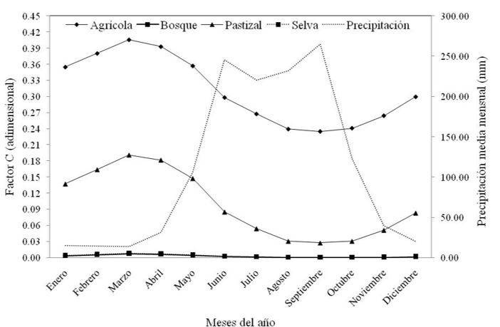
Figure 4 shows the graphic distribution of monthly average NDVI by type of coverage. Figure 5 shows the graphic distribution of the C factor values by type of vegetation cover. It should be noted that, although the NDVI values are similar between forest covers to those of herbaceous covers, the value of C is not the same, given the behavior of the vegetation before the kinetic energy of rain. The values of the factor C oscillate in the ranges of 0.002 to 0.003 for forest and jungle and 0.04 to 0.8 for agricultural use (Figure 6).


Current water erosion (EHA)
Figure 7 shows the spatial distribution of the annual water erosion calculated in the study area, the results indicate that 73% of the basin presents some degree of erosion, the moderate degree has a higher incidence (34%). Approximately 9% (58 265 ha) show a very high degree of erosion. These predictions are consistent with those obtained in the National Baseline for Land Degradation and Desertification (UACH-CONAFOR, 2013).

The monthly values of erosivity of rain and vegetation cover, allow us to observe a clear seasonality regarding these two dependent factors, since, although rain is the ‘aggressive’ agent in the process, it is also the one that allows the development of the vegetation cover, the latter being the factor with the greatest mitigating capacity for erosion. The assigned values given the characteristics of the soil and the topography, remained constant, given the difficulty for these conditions to change in the short term (Table 3).
Table 3 Monthly water erosion in the Sumidero Canyon Basin.
| Month | EHA (t) | Values per hectare per year | ||
| Average EHA | (m-3) | (Cm) | ||
| January | 131 002.614 | 0.196 | 0.15 | 0.002 |
| February | 94 409.056 | 0.141 | 0.108 | 0.001 |
| March | 187 090.203 | 0.279 | 0.215 | 0.002 |
| April | 831 494.091 | 1.241 | 0.955 | 0.01 |
| May | 2 633 999.18 | 3.931 | 3.024 | 0.03 |
| June | 7 021 906.936 | 10.48 | 8.062 | 0.081 |
| July | 5 074 980.012 | 7.574 | 5.826 | 0.058 |
| August | 4 661 919.286 | 6.958 | 5.352 | 0.054 |
| September | 5 012 810.799 | 7.482 | 5.755 | 0.058 |
| October | 1 612 757.614 | 2.407 | 1.852 | 0.019 |
| November | 411 623.851 | 0.614 | 0.473 | 0.005 |
| December | 134 357.542 | 0.201 | 0.154 | 0.002 |
| Total | 27 808 351.184 | 41.504 | 31.926 | 0.319 |
The month in which water erosion is greatest is June, in total 7 021 906.94 t are lost, an average of 10 480 t ha-1 year-1 (5 400 369.26 m3 year-1). The average EHA reflects the average rate of soil degradation due to water erosion, it should be clarified that this value is different from what in various publications refers to specific degradation, since this concept is applied when considering the production of sediments per unit of area. Likewise, the average values of cubic meters are the relationship between the EHA in tons per hectare, transformed into cubic meters considering an apparent density of 1.3 t m-3.
The behavior of the EHA from June compared to May, to July and September, is given by the amount of rain each month, but mainly by the state of the vegetation cover: from May to June there is an increase of around 5 million t of eroded soil, a situation which, in September, with rainfall values similar to June, due to its greater vegetation cover, reduces erosion by approximately 2 million t. The foregoing indicates the importance and feasibility of improving the vegetation cover of the soil, which represents considerable decreases in the susceptibility of the soil to be eroded, with respect to the mechanical practices aimed at controlling water erosion.
The annual average erosion in the basin is 41.5 t ha-1 year-1. According to SEMARNAT and UACH, (2003) the Sumidero Canyon Basin is losing 9 times the allowable rate for Mexico. Comparing with the estimate of global water erosion (75 x 109 t year-1; Pimentel et al., 1995), the Sumidero Canyon basin is predicted to contribute 0.04% of global erosion.
Conclusions
From the results of the present study, it is concluded that RUSLE is an effective model for both quantitative and qualitative evaluation of soil erosion for watershed conservation management.
Based on available information on topography, soils, land use and the temporal analysis of data series, as well as remote sensing techniques and geographic information systems, a methodology has been developed that allows estimating water erosion on slopes at level national.
In this study, the RUSLE model was used, using an average monthly base, the appropriate calculation of erosion and coverage factors for each month, to obtain the erosive potential of rainfall and runoff in each given period of time. The slope steepness factor is best calculated using high resolution MDE.
GIS has provided a very useful platform to carry out the task of collecting, processing, displaying and analyzing data. Its benefits include updating data, data management and presenting the data in the most appropriate way according to the user’s needs. It seems clear that maintaining an adequate vegetation cover in critical areas would be enough to minimize and even eliminate erosive processes related to water erosion.
Literatura citada
Cortés, T. H. G. B.; Figueroa, S. C. A.; Ortiz, S. y González, F. V. C. 1992. Caracterización de la erosividad de la lluvia en México utilizando métodos multivariados. 1. Descripción de intensidades máximas e índices de erosividad de la lluvia. Agrociencia. 3(2):115-138. [ Links ]
UACH-CONAFOR. 2013. Comisión Nacional Forestal y la Universidad Autónoma Chapingo. Línea Base Nacional de Degradación de Tierras y Desertificación. 146-147 p. [ Links ]
CP. 1991. Colegio de Postgraduados. Manual de conservación del suelo y del agua: instructivo. Tercera edición. CP. Cha pingo, Texcoco, Estado de México. 3-6 pp. [ Links ]
Ganasri, B. and Ramesh, H. 2015. Assessment of soil erosion by RUSLE model using remote sensing and GIS - A case study of Nethravathi Basin. Geoscience Frontiers. 7(6):953-961. [ Links ]
Hickey, R.; Smith, A. and Jankowski, P. 1994. Slope length calculations from a DEM within Arc/Info GRID. Computers, Environment, and Urban Systems. 18(5):365-380. [ Links ]
Hickey, R. 2000. Slope angle and slope length solutions for GIS. Cartography. 29(1):1-8. [ Links ]
Hua, L.; Gallant, J.; Prusser, I. P. and Pristley, G. 2001. Prediction of sheet and rill erosion over the Australian Continent, incorporating monthly soil Loss distribution. CSIRO Land and Water, Technical Report. 30 p. [ Links ]
INEGI. 1977. Instituto Nacional de Estadística y Geografía. Cartas edafológicas E15C77, E15C87, E15C68, E15C78, E15A18, E15C59, E15C69, E15C79, E15C89, E15D51, E15D61, E15D71, E15D62 y E15D72. Escala 1:50 000, 1a. (Ed.) México, DF. [ Links ]
INEGI. 2011. Instituto Nacional de Estadística y Geografía. Continúo de elevaciones mexicano CEM (2.0). [ Links ]
IMTA. 2006. Instituto Mexicano de Tecnología del Agua. Extractor rápido de información climatológica ERIC III. CD ROM. México, DF. [ Links ]
Mol, J. H. and Oubote, E. 2004. Downstream effects of erosion from small-scale gold mining on the instream habitat and fish community of a small neotropical rainforest stream. Conservation Biol. 18(1):201-214. [ Links ]
Morgan, R. P. C. 1997. Erosión y conservación del suelo. Urbano, T. P. y Urbano, L. J. de M. de M. (Trad.). Mundi-Prensa. 343 p. [ Links ]
Pacheco, H. 2012. El índice de erosión potencial en la vertiente norte del Waraira Repano, estado Vargas, Venezuela. Cuadernos de Geografía. Rev. Colomb. Geog. 21(2):2256-5442. [ Links ]
Pimentel, D.; Harvey, C.; Resosudarmo, P.; Sinclair, K.; Kurs, D.; McNair, M.; Crist, S.; Shpritz, L.; Fitton, L.; Saffouri, R. and Blair, R. 1995. Environmental and economic costs of soil erosion and conservation benefits. Science. 267(5201):1117-1123. [ Links ]
Renard, K. G., Foster G. R., 1994. RUSLE revisited: status, questions, answers, and the future. J. Soil Water Conserv. 49(3):213-220. [ Links ]
Renard, K. G.; Foster, G. R.; Weesies, G. A.; McCool, D. K. and Yoder, D. C. 1997. Predicting soil erosion by water: a guide to conservation planning with the revised universal soil loss equation (RUSLE). USDA, agricultural research service, agriculture handbook. No. 703. US. Washington, District of Columbia, USA. 404 p. [ Links ]
Rosewell, C. J. 1993. SOILOSS. A program to assist in the selection of management practices to reduce erosion. Technical Handbook No. 11 2nd (Ed.). Soil Conservation Service of NSW, Sydney. 86 p. [ Links ]
SEMARNAT-UACH. 2003. Secretaría de Medio Ambiente y Recursos Naturales y la Universidad Autónoma Chapingo. Evaluación de la pérdida de suelos por erosión hídrica y eólica en la República Mexicana, escala 1:000 000. 145 p. [ Links ]
Van-Remortel, R. D.; Maichle, R. W. M. E. and Hickey, R. J. 2004. Computing the LS factor for the revised universal soil loss equation through array-based slope processing of digital elevation data using a C. executable. Computers Geosciences. 30(9-10):1043-1053. [ Links ]
Wishmeier, W. H.; Hohnson, C. B. and Cross, B. V. 1971. A soil probability monograph and farmland and construction sites. Soil Water Conservation. 26(5):189-193. [ Links ]
Wischmeier, W. H., and Smith.D. D. 1978. Predicting rain fall erosion losses: a guide to conservation planning. USDA. SEA. Agriculture Handbook 537. Washington, DC. 58 p. [ Links ]
Received: June 01, 2020; Accepted: October 01, 2020
 Este es un artículo publicado en acceso abierto bajo una licencia
Creative Commons
Este es un artículo publicado en acceso abierto bajo una licencia
Creative Commons
