


Serviços Personalizados
Journal
Artigo
 texto em
  Inglês (pdf)
 Artigo em XML
 Referências do artigo
 Enviar este artigo por email
Indicadores
-
 Citado por SciELO
 -
 Acessos
Links relacionados
-
 Similares em
SciELO
Similares em
SciELO
Compartilhar

 Permalink
Revista mexicana de ciencias agrícolas
versão impressa ISSN 2007-0934
Rev. Mex. Cienc. Agríc vol.11 no.6 Texcoco Ago./Set. 2020 Epub 11-Out-2021
https://doi.org/10.29312/remexca.v11i6.2513
Articles
Private agricultural insurance model for small agricultural producers in Mexico
1Posgrado de Economía Agrícola-Universidad Autónoma Chapingo. Carretera México-Texcoco km 38.5 Chapingo, Estado de México. CP. 56230. (rocioayvar@yahoo.com.mx; ramirezrocio67@hotmail.com).
2Campo Experimental Valle de México-INIFAP. Carretera Los Reyes-Texcoco km 13.5, Coatlinchan, Texcoco, Estado de México, México. CP. 56250. Tel. 01 800 0882222, ext. 85353. (dsangerman@yahoo.com.mx).
The Federal Government has encouraged the practice of agricultural insurance with subsidies to the producers who use these services, but the way in which expenses have been channeled to strengthen the practice of insurance has not been sufficient to achieve, especially among small producers, generalize this practice. The objective of this research was to propose a model of agricultural insurance, whoever acquires it receives additional benefits to those that normally exist and are obtained in traditional insurance, in the year 2018. The methodology starts from the theoretical principle of Burns’ economic cycles and Mitchell which is one of the first time series studies of business cycles based on Avella-Gomez and Ferguson. With the statistical regression technique applied to production and yield data of the basic crop, for this case white corn, modeled with the Statistical Analysis System (SAS) program. Some results and conclusions observed were that unlike traditional insurance, it is proposed that the amounts to be paid for insurance premiums be determined before each agricultural cycle, with field information obtained by specialists and government technicians who are more close to the producers. It is considered that different amounts of insurance premium should be determined by agricultural region of the Rural Development District, by crop and by irrigation or temporary water regime.
Keyword: agricultural insurance; small producers; yields
El Gobierno Federal ha incentivado la práctica de seguros agrícolas con subsidios a los productores usuarios de estos servicios, pero la forma en que han sido canalizados los gastos para fortalecer la práctica de los seguros no ha sido suficiente para lograr, sobre todo entre productores pequeños, generalizar esta práctica. El objetivo de esta investigación fue proponer un modelo de seguro agrícola, quien lo adquiere recibe beneficios adicionales a los que normalmente existen y se obtienen en los seguros tradicionales, en el año 2018. La metodología parte del principio teórico de los ciclos económico de Burns y Mitchell el cual es uno de los primeros estudios de ciclos económicos basado en series de tiempo de Avella-Gómez y Ferguson. Con la técnica estadística de regresión aplicada a datos de producción y rendimientos del cultivo básico, para este caso el maíz blanco, modelado con el programa Statistical Analysis System (SAS). Algunos resultados y conclusiones, observados fueron que a diferencia de los seguros tradicionales, se propone que los montos a pagar por concepto de primas de aseguramiento, se determinen antes de cada ciclo agrícola, con información de campo obtenida por especialistas y técnicos gubernamentales que están más cerca de los productores. Se considera que se deben determinar montos diferentes de prima de seguro por región agrícola de los Distrito de Desarrollo Rural, por cultivo y por régimen hídrico de riego o temporal.
Palabra clave: pequeños productores; rendimientos; seguro agrícola
Introduction
One of the most important instruments for the primary sector is agricultural insurance due to the fact of covering possible losses due to adverse climatic effects, in addition to stabilizing income, among other effects (Agroasemex, 2016). The various public policy approaches have tried various modalities to provide agricultural insurance to small and medium producers, which have gone from a state monopoly to the participation of private insurance companies, in all subsidies are present to a greater or lesser extent (Díaz-Tapia, 2006). This has allowed Mexico to be one of the developing countries with advanced insurance schemes (FAO, 2018).
Despite the efforts made to incorporate producers into the initiative to insure their production, external evaluations of government assurance programs show that producers, especially temporary and with small areas, have not adopted assurance programs (AMUCSS, 2014), due to the way they operate, they are difficult to access for smallholder agricultural producers, although they are also little accepted and practiced by medium and even large producers, data from ENA (2017) show that only 5% of UP, they had a policy of some type of insurance, evidenced by a low demand, of which 98% refer to small and medium producers. Insurance has been used more for financing or imposing government agencies to protect itself from risk than for the very purpose of strengthening the culture of agricultural risk protection to protect the income of producers (Díaz-Tapia, 2006).
Among the factors that limit the acquisition of agricultural insurance are the costs of the insurance premium (AMUCSS, 2014), in addition to a high rejection for not complying with all the requirements requested by credit institutions (ENA, 2017), together with this, the producer does not perceive beneficial to pay the insurance premium cycle by cycle and receive only compensation from the insurance entity in the agricultural cycle where it has a catastrophic event, which in many cases only covers the amount of production costs, but not the total value of the lost product. It is in this aspect that work must be done to make them of greater interest to producers and it is at this point that the focus of this work is focused.
Agricultural producers, especially those of staple and seasonal crops, annually face ups and downs in their product quantities that are reflected with accelerating effects on the instability of their income over time FIRA (2016). When the temporal is good and they obtain high quantities of product, the price of the same decreases due to excess supply and they face a negative effect on their income. When the temporal is bad, the price of the product rises, but the producer has little product to offer to the market and therefore also low income. The instability of income that occurs from one year to the next causes many producers in the medium term to abandon the activity and even more serious, when there is a total loss of the crop due to the presence of unfavorable climatic conditions, they tend to abandon agriculture and emigrate accelerating the imbalance between supply and demand of the agricultural product and its negative effects. Therefore, insurance not only helps reduce risks, but also reduces the imbalance between supply and demand (FAO, 2018b).
However, this serious problem in agricultural production processes and the worsening of the practice of insuring their crops against climatic events is very rare among farmers in Mexico, especially among the so-called small producers (up to 10 ha) that constitute 71.23% (ENA, 2017).
The objective was to propose an agricultural insurance scheme that offers the small producer better benefits than those provided with the current schemes, which are attractive and viable for small producers. An agricultural insurance model that provides stability of income for agricultural producers, which results in a significant decrease in emigration from the countryside to the city or abroad. The hypothesis proposed is that a wide variation in annual income around a trend line in a medium and long-term cycle causes a decreasing trend of growth in the value of agricultural production, generating an increase in the phenomenon of emigration and abandonment of productive land which in turn causes a decrease in the growth of the value of production and restriction in the growth of the supply of food products generated in the field.
It is possible to facilitate access to the practice of agricultural insurance to low-income producers, through a model in which the insurance premium is managed requiring less financial effort for small producers and that minimizes the wide variation that occurs in their income.
Materials and methods
The methodology starts from the theoretical principle of the economic cycles of Burns and Mitchell (1946), which is one of the first studies of economic cycles based on time series (Avella-Gómez and Ferguson, 2004). The main instrument used to calculate the cost of the premium and determine the agricultural cover is the statistical regression technique applied to production and yield data of the basic crop (in this case white corn), modeled with the Statistical program. Analysis System (SAS, 2001).
According to the cycle theory, applied to agricultural production, even when the climatic conditions are good and high product levels are obtained, there is a decrease in its price due to excess supply, which negatively impacts the trend and the orients towards a decrease in the income of the producer. If the climatic conditions are unfavorable, there are high prices of the product in the market due to the low production that results in a decrease in the offer and affects the producer’s low income because he owns little product to offer to the market, so his income also tends to be low (González et al., 2018; Sangerman-Jarquín et al., 2018).
If these variations are strong and continuous, the consequence is that many of the producers tend to abandon the activity and in the medium term the supply of agricultural products is diminished and does not respond to the needs of the growing demand driven by the constant increase in the consumer population. It has been shown that, in the economy of a country, in the medium and long term, if the annual variation in the value of production is wide, the growth rate of production is low and becomes negative, while, if those variations are moderate, the
annual growth rate of the product tends to be higher. Therefore, the measures to be applied to reduce the high variation in producers' incomes are those that favor greater stability in annual income.
The theoretical principle of business cycles is applicable to separate products. If data from annual corn production in Mexico are observed and a trend line is drawn, it can be seen that during the period in which the production data moves further from the trend line (income instability in the period (2008- 2012) the trend line shows a growth rate not only lower but in this case the growth trend becomes negative, while in the previous period (2000-2008) where the variation is moderate, the line shows a trend to the rise in production (Figure 1). Figure 1 shows an increasing trend in corn production in the first years 2000-2008 and a decreasing trend in recent years, and also, as can be seen, the period final is associated with greater instability of production (Spielman et al., 2011).

Figure 1 Behavior of corn production in Mexico period (1998-2018). Elaboration with data from SIAP (2020).
The trend of instability and negative growth in production, such as that observed in the period 2008-2011, can be reversed towards sustained growth if greater stability is given to producers' incomes. In this case, it is understood that a trend is stable if the values observed each year do not differ significantly from the values of a trend line that can be horizontal when the production of a good remains at the same production level over time or as it is desirable, in terms of growth, the trend line is presented with a positive slope. In order to achieve better stability in the income of producers; therefore, in the quantities of food that go on the market, an insurance system is proposed in which the producer pays an annual premium to the insurer and receives compensation from the insurer in the years in which its production falls below of the trend line of yields in production (SIAP, 2014).
Public policy provision. Given the practically null response of expected results to generalize the use of agricultural insurance especially for very small agricultural producers, a call was issued by the Federal Government, to propose mechanisms and designs of crop insurance models that are attractive to producers to increase this practice. A characteristic of the proposed insurance mechanisms is that it is in the genuine interest of the producers and that therefore they are the ones who pay the insurance instead of waiting for government institutions to cover this cost, a measure
that until now has not had positive results in their attempt to promote the culture of agricultural insurance among small producers and smallholders who constitute the vast majority in the country. It is a governmental disposition that the instance or instances that operate the insurance system are private companies, as referred to by authors such as Engle (2001); Díaz-Tapia (2006). The participation of the Federal Government must be marginal in terms of financing and that it is fundamentally under the legal control of the insurance companies in that they have to be duly registered in the corresponding instances of the government and under the rules established for the operation of private insurers.
Only, it must be an active participation of the Federal Government; through its instances in the field: Rural Development Districts (DDR) and Rural Development Care Centers (CADER) CADER (2018); DDR (2018) provide crop yield data for agricultural insurance operation areas.
Characteristics of the proposal derived from the present investigation
The characteristics of the investigation are detailed below: a) the insurance coverage guarantees, at least, the income corresponding to the value of the product marked by the trend line for each year of operation; b) the insurance premium is calculated by the average of the yield differences obtained in previous years with respect to the values indicated by the trend line; c) the trend line should be updated each year, eliminating the first year of the period analyzed and adding the actual yield data obtained the last year in which the insurance was exercised (not the predicted one, but the real one); d) the insurance premium must be paid in real terms (measured in kg of product at the price in force at the time the premium is paid to the insurer); and e) the value of the insurance premium must be equal to the average of the deviations of production per hectare from the trend line in a historical period of 10 or 12 years, multiplied by the current average rural price.
Insurers must consider at least one year of disastrous consequences for the crop, if it does not exist in the period analyzed, include the yield of the year prior to the series of years where there was a highly significant loss and their respective crop yields. This data will obviously raise the value of the premium to be paid, but it is very likely that the insurer will demand that it be established in this way to cover catastrophic cases and thus run a shared risk between producers and the insurance company.
The insurer’s argument for claiming the above detail in the calculation of the insurance premium is that, if there is not a year of very low returns in the entire 10-year period analyzed, the probability that this phenomenon will soon exist is highly probable. The insurer’s proposal would be that if in the period of 10 or 12 years, a catastrophic year does not appear, include in the series the yield of the most recent year in which this very low yield characteristic was obtained. The previous measure can be used as an option to determine two insurance premiums with different costs: one with insurance against catastrophic loss of production and the other with a lower cost that only covers losses not greater than the one with the lowest drop in yield in the period analyzed (Engle, 2001; Spielman et al., 2011).
In the event that the yield obtained at the end of the planting and harvesting period is less than the expected yield, marked by the trend line, the difference will be covered by the insurance company and in an amount equivalent to the value of that difference at prices of the grain prevailing on the payment date. If the yield is higher than the one indicated by the trend line, the insurance company will not contribute any compensation to the producer. Secondary to the above characteristics, the assurance process proposed by the insurer may have other options to be chosen individually by the producers.
It must be totally valid to issue different insurance premium values also for the same product, in the same region, for example: an insurance premium for irrigation corn and another for seasonal corn within the same DDR (2018). given that their respective variations in yield should be different and most likely of lesser magnitude in the irrigated lands. If it is the case that it is recognized that in the same crop under the same conditions of water regime there are different behaviors in yields between CADER of the same DDR and thus agreed between producers and insurance company, with supervision of the Heads of CADER, the insurance premium may also be differentiated by CADER (2018).
In the latter case, the insurance premium amounts must be calculated with their respective yield trend lines in each of the CADER (2018). If not, its monetary value, calculated with the averages of the variation of yields with respect to the trend line, can be objected by irrigation corn producers who can claim to pay a lower insurance fee because the variation in yields with regarding the trend line in irrigation, it cannot be as large as that presented in temporal conditions within the same DDR or CADER.
In the same way, some other factor may arise that forces differentiation of insurance premiums for the same crop within the same CADER. For example, the cultivation carried out under the traditional process and the one carried out with the incorporation of technology. In all these cases, the insurance premium quotas can be differentiated, always with the agreement of producers, insurance companies and supervision of public officials in the agricultural area. In general terms, it is recommended that a private body take over the administration of the insurance and that differentiated insurance payments be made for the spring-summer (SS) and autumn-winter (AW) cycles by water regime (irrigation or temporary) by cultivation, by technological level (technified and non-technified) by CADER and by some other criterion that results and that justifies the differentiation of insurance premiums.
Field data on yields for calculating insurance premiums must be provided by DDR staff and, where appropriate, by CADER staff.
Participation of the insurance company. Insurance companies are sure to take precautions for government officials to provide reliable figures, while producers in the area will do the same. These data must take into account the current prices of the products in the agricultural area. All this should lead to having better field information statistics to be used in this and for other purposes, OECD (2018).
The insurance company’s business is that at the beginning of an agricultural cycle it receives money from the producers for the insurance premium, at the end of the cycle and only if the production falls below the expected yield, indicated by the trend line, pays the producer the product difference obtained. In these cases, the insurance authority returns money to the producer after keeping it in its possession throughout the production cycle, which represents the collection of monetary resources that it can use for other financial businesses during that period of time without paying interest (CADER, 2018; DDR, 2018).
In the event that the yield is higher than expected by the trend line, not only does it not pay interest, but it keeps all the premium payment. In the medium and long term, only half of the resources obtained by payment of insurance premiums return to the producer, the rest remains as income of the insurer for providing the service, in addition to profits obtained from managing all the resources. that are temporarily in your possession and that you can invest in activities complementary to the crop insurance business.
In both cases, the insurance company obtains financial benefits of a magnitude determined by the number of producers, the area insured in each agricultural cycle and the magnitude of variation in yields. For the first two aspects directly linked to the financial amounts it obtains, it is convenient for it to be the main promoter of this type of insurance.
Reiterating that the insurance premium per hectare planted to corn, must be processed with the yield data per hectare observed in a period that contains a year of loss considered disastrous or catastrophic, which the insurance company will surely require, to guarantee what the average value of the annual insurance premium, a resource is being obtained to cover this eventuality, the above reaffirmed research by Hartwich and Scheidegger (2010).
Do not forget to consider that there may also be years in which the yields were exceptionally high and that they would present points far from the trend line that would increase the average of the variations and consequently the value of the insurance premium in favor of the company insurance carrier. This is also left as a point to be agreed between DDR authorities (supporting producers) and insurance company personnel. The agreement would be based on whether or not to remove this data from the series of years analyzed to determine the value of the risk premium (De Martinelli, 2012).
Producer participation. i) accept and make the payment of the insurance premiums at the beginning of the agricultural cycle; ii) collaborate by participating and endorsing the yield data of the insured products obtained by CADER and DDR personnel; iii) allow obtaining and ratification of yield data when requested by the insurance company and by the corresponding CADER; iv) Federal Government participation; v) authorize the insurance companies to carry out their activities after formal registration of the same, before the corresponding governmental instance; vi) provide the applicable norms to exercise the assurance service to private institutions and DDR and CADER personnel; vii) provide the definitive returns information by DDR and CADER; through these instances, by crop, by agricultural cycle, by technological level and by any other variant of crop conditions that allows identifying the specific insurance quotas or premiums for the selected conditions; viii) provide companies through CADER with current price data for crops in the region where the insurance system operates, which may be verified in the field by the company or by the producers; xi) supervise and authorize the insurance entity, the variants requested to differentiate the insurance premiums; and x) advantages over the traditional agricultural insurance system (Rivas, 2014; CADER, 2018; DDR, 2018).
Producers each year pay the insurance premium but every 2 years, on average, they receive a refund of resources (when their production falls below the trend line) which means that in the long term, they only pay half of the agricultural insurance expenses because the other half of the payments are returned to them when they are most needed because they are received in low yield years -below the trend line- and at the same time it is helping to significantly reduce the high instability of producers' income and more regular income security, to remain in better conditions in the agricultural activity FAO (2018a).
In this way, according to the theory of business cycles, this reduction in production variability positively influences the growth rate of total production. In the medium and long terms, stability in the value of production should contribute to raising the growth rate of production of agricultural goods SAGARPA (2013).
An additional benefit of substantial importance is that it contributes to retaining producers in their activity to obtain a greater increase in the production of goods and at the same time meet the growing demand for food driven by the growth of the consuming population. Although by reducing the risk of large variations in production and these are lower in cost and reinforce the safety and tranquility of the producer, the adoption of the insurance system may migrate towards the practice of market hedges in the agricultural stock market.
The administration of the insurance by private entities does not require payments to the insurance company or government subsidies. Its benefit is obtained from collecting money from the producers and returning it at a later time without paying interest and with all the benefits that this means for any financial company that collects money from the participating public without paying interest.
Results and discussion
With data from one of the most common crops, irrigation corn in the 2008-2018 period with a projection of the expected yield for 2019 in the DDR Tejupilco, located in the State of Mexico, with yield data expressed in tons per hectare and where the annual variation of yields is relatively high and has a horizontal trend; that is, there is no tendency to increase production in the period analyzed, as observed by Gamboa (2010).
The processing of the information to obtain the values of the insurance premiums can be carried out in any computational package that contains the process of regression and projection of data, over time (Ayvar et al., 2018; FIRA, 2016a; FIRA, 2016b).
In the Statistical Analysis System (SAS, 2001), to obtain the trend line and the deviations of the observed data with respect to the data predicted with the trend line, they were obtained with the following program.
DATA MAIZ;
INPUT T R; T2=T¨T;
CARDS;
2009
3.00
2018
2.29
2019 ,
PROC GLM; MODEL R=T T2/PREDICTED; RUN;
Program description. On the first line, with the DATA MAIZ statement; a name is assigned to the data to be processed: MAIZ. The INPUT indication indicates that the variables T (year) and R (tons of corn) enter the database, and in that order of the columns. T2= T*T, with this expression it is requested that the variable be generated with a value equal to the square of the values of the variable T, which is identified with the name of T2. This generated variable is used to identify and apply a quadratic regression model in case it is observed that the yield data in a graph is dispersed with a curvature and not as a straight line, which can be seen visually on the graph. dispersion of the yield data that will be processed or through the regression result, where it is identified that there is no curvature in the line if the coefficient of the quadratic term T2 is equal to zero.
In the same way, you can add a variable T3 that is generated with the instruction T3=T2*T; if the data series appears to have two concavities in the period analyzed. CARDS, this instruction indicates that the data to be processed is immediately incorporated. Next, the data to process of the two variables appear and in the order in which they appear in the INPUT (first T and then R). A future year 2019 is included, which does not contain yield data and a point is placed in the corresponding yield value. After the information for each year, including the 2019 yield point that is not available, a is placed ; (semicolon) to indicate that the data to be processed ends there.
PROC GLM; MODEL R=T T2/PREDICTED, with this instruction it is requested that a general linear model regression process (GLM) be carried out, with the dependent variable R of yield as a function of the independent variables T and T2, for its part/PREDICTED instruction indicates that a yield prediction is made for the year 2019 that does not have data, which is done with the trend line corresponding to the model of the function R= f(T, T2) prepared in this same (Prayag et al., 2010).
At the same time, it is requested that the predicted values be generated, corresponding to each production data of each year, located in the trend line and the corresponding differences expressed in negative values for the production data that remain below the trend line and positive for the value differences that are above the trend line, this is indicated in Table 1. Only with an ENTER, the requested program is executed and the information generated in the computer’s output sheet is generated.
Table 1 Results of the output sheet.
| Parameter | Estimate | Standard error | Value t | Pr > |t| | |
| Intercept | 197.0192727 | B | 67.2233714 | 2.93 | 0.019 |
| T | -0.0965455 | B | 0.03338629 | -2.89 | 0.0201 |
| T2 | 0 | B | - | - | - |
Elaboration with data from SIAP (2020); SAS (2001).
These results indicate that the regression adjusts the processed data to a straight line with ordinate to the origin of 197.0192727 a coefficient for the yield variable of -0.096 and the regression coefficient for the variable T2 is zero, so the data presents a line of trend that has no concavity and is a straight line.
Therefore, the function is: R = 197.0192727 - 0.0965455T. Next and as a product of the /PREDICTED option included in the computer program, the data in the following table is generated where they appear: a variable indicating the progressive number of the processed data (observed). The data corresponding to each annual yield value in the trend line prepared by the program, including the prediction for the year 2019 of which only the year was included and a point as missing data (predicted) and the vertical differences between the data of processed yields and their corresponding value of difference with the trend line, as observed in (Table 2). With a negative sign for those below the line and positive for those above the line (residuals).
Table 2 Observed, predicted and residual yield data by observation.
| Observations | Observed | Predicts | Residual |
| 1 | 3 | 3.05945455 | -0.05945455 |
| 2 | 2.86 | 2.96290909 | -0.10290909 |
| 3 | 3.28 | 2.86636364 | 0.41363636 |
| 4 | 2.98 | 2.76981818 | 0.21018182 |
| 5 | 2.59 | 2.67327273 | -0.08327273 |
| 6 | 2.2 | 2.57672727 | -0.37672727 |
| 7 | 2.25 | 2.48018182 | -0.23018182 |
| 8 | 2.07 | 2.38363636 | -0.31363636 |
| 9 | 2.73 | 2.28709091 | 0.44290909 |
| 10 | 2.29 | 2.19054545 | 0.09945455 |
| 11 | - | 2.094 | - |
Elaboration with data from SIAP (2020); SAS (2001).
Note that line number 15 corresponds to the year 2019 in which your estimated yield data for that year appears. From the previous table of results, it can be verified that the values that fall below the trend line (residuals with negative values) added together in their absolute values, must be equal to the sum of the positive values that remain above the line. of trend. It can also be corroborated that the sum of the positive and negative values is equal to zero, which confirms the previous statement (SAGARPA, 2013; FIRA, 2016).
In this case of years analyzed in even numbers, the insurance premium can be obtained by the average of the negative values (in absolute terms) or by the average of the positive ones. Not so in the event that the process is carried out with a non-number of years analyzed because although the sums of the absolute values of the negatives are equal to the sum of the data of positive values or deviations, the average would be less in the series of positive or negative data that has a greater number of years (Table 3).
Table 3 Annual returns per year, observed and predicted 2009-2019.
| Year | Observed | Predicted |
| 2009 | 3 | 3.059 |
| 2010 | 2.86 | 2.963 |
| 2011 | 3.28 | 2.866 |
| 2012 | 2.98 | 2.77 |
| 2013 | 2.59 | 2.673 |
| 2014 | 2.2 | 2.577 |
| 2015 | 2.25 | 2.48 |
| 2016 | 2.07 | 2.383 |
| 2017 | 2.73 | 2.287 |
| 2018 | 2.29 | 2.19 |
| 2019 | - | 2.094 |
Elaboration with data SIAP (2020).
In this case, the general average of the residual values must be taken, previously converting the negatives into positives. Converting the following numerical results obtained, including the prediction of yield for the year 2019, in Figure 2 it is expressed as follows.
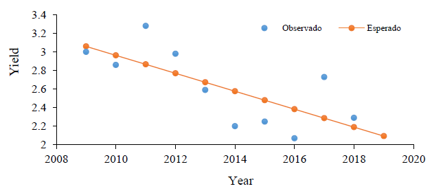
Figure 2 Observed and estimated yield of corn under irrigation in the DDR Tejupilco 2009-2018 and projection to 2019. Elaboration with data from SIAP (2020).
It will be appreciated that the estimated regression line shows a slight downward trend as indicated by the negative coefficient of the analyzed variable (T) and that this trend is in line with a relatively wide variation in yields in the period analyzed, so that the insurance premium will be high so long as this instability of returns is not moderated.
The average of the deviations of the yields with respect to the trend line in this case is from 0.391 to 391 kg which are valued at a hypothetical price of 3 pesos per kg as the price when paying the insurance premium in the year 2019, this would amount to 1 174 pesos per hectare (Hartwich and Scheidegger, 2010; Rodríguez, 2017).
Recommendations
The cost or premium of agricultural insurance must be covered by the producers, without government subsidy. With what the insurer returns in one year, you are better able to pay the premium for the following year.
Unlike traditional insurance, the amounts to be paid for insurance premiums are determined before each agricultural cycle, with field information obtained by specialists and government technicians who are closer to producers, CADER and DDR personnel. Private insurance operating companies must be duly registered with the Federal, State or corresponding government according to current insurance legislation. The agricultural insurance premium must be differentiated by region, by crop, by agricultural cycle A-W and S-S, by water regime (irrigation and temporary) by technological level (technical and non-technical) and by CADER. If there is an agreement between the insurance company, producers and supervisory authorities, it can be differentiated by criteria based on factors that affect yields per hectare.
The calculation of the insurance premium must be in real values, based on data on the variation in yields in kg ha-1 valued at prices in effect at the time the premium is paid. In the production cycle in which the yield is less than the predicted data, the insurer’s remuneration towards the producer must be equal to the monetary value of the difference between expected yield and yield obtained at current prices of the product at the time of delivery of retribution.
If the return obtained is of a higher value than that predicted by the trend line, the insurance office does not pay the producer anything. The insurance premium must be equal to the average of the differences between the returns obtained and the corresponding returns in line with their trend, using a period of 10 or 12 years. To calculate the insurance premium, the analyzed time series must be updated. Each year, the data for the first year will be removed from the annual yield data series and the actual yield for the forecast year will be added. If the yield obtained is below that predicted by the trend line, the insurer must pay what results from that difference in yield multiplied by the price of the product in force at the time of the insurer’s payment to Engle producers (2001).
Conclusions
The designed agricultural insurance model guarantees to provide greater stability of income for agricultural producers and in terms of cost, it turns out to be much lower than the fees paid to insurers currently. With this agricultural insurance structure, over time, the producer receives re-entries of value equal to half of what he delivers each year to insurers. And you get it when it’s needed most, the year it performs below the trend line.
The stability in income of producers must have a decisive influence on their permanence in the work of food production and, in turn, influence the permanence of the population in their places of origin. With the proposed agricultural insurance model, those who acquire this service receive additional benefits to those normally obtained in traditional insurance, which is that at least every two years, they receive an income similar to the premium they pay for be insured against loss of your crops. What, in the medium and long term, the number of effective payments of insurance payments is reduced by half. Given the additional benefits indicated, the model is more attractive and viable for small producers, which should contribute to the purpose of generalizing the practice of agricultural insurance.
Literatura citada
AGROSEMEX. 2016. Diagnóstico programa presupuestal S 265. Programa de aseguramiento agropecuario. Documento interno. 57 p. [ Links ]
AMUCSS. 2014. Asociación mexicana de unidades de crédito del sector social AC. 19 pp. https://issuu.com/amucss/docs/documento-ve-agricola-vl. [ Links ]
Avella-Gómez, M. y Fergusson, T. L. 2004. El ciclo económico-enfoques e ilustraciones-los ciclos económicos de Estados Unidos y Colombia. Borradores de Economía 002465. Banco de la República. [ Links ]
Ayvar, V. Ma. Del R. Pérez, Z. A. y Portillo, V. M. 2018. Seguro para pequeños productores de maíz en el estado de Puebla. Rev. Mex. Cienc. Agríc. 9(4):761-772. [ Links ]
Burns, A. F. and Mitchell, W C. 1946. Measuring business cycles. New York. National Bureau of Economic Research. ISBN 978-0-87014-085-3. 560 p. [ Links ]
CADER. 2018. El Centro de Aprendizaje para el Desarrollo Rural (CADER)-Secretaría de Agricultura, Ganadería, Desarrollo Rural, Pesca y Alimentación. Componente de atención a siniestros agropecuarios. https://www.gob.mx/sagarpa/acciones-y-programas/ componente-de-atencion-. [ Links ]
DDR. 2018. Distritos de Desarrollo Rural (DDR)-Secretaría de Agricultura, Ganadería, Desarrollo Rural, Pesca y Alimentación. Componente de atención a siniestros agropecuarios . https://www.gob.mx/sagarpa/acciones-y-programas/componente-de-atencion-asiniestros-agropecuarios. [ Links ]
De Martinelli, G. 2012. De los conceptos a la construcción de los tipos sociales agrarios, una mirada sobre distintos modelos y las estrategias metodológicas Argentina.. Rev. Latinoam. Metodol. Inves. Soc. 2(1):24-43. [ Links ]
Díaz-Tapia, A. 2006. El seguro agropecuario en México: experiencias recientes serie: estudios y perspectivas. Unidad de Desarrollo Agrícola Naciones Unidas. México, DF. ISBN:92-1-322991-7. 237 p. [ Links ]
ENA. 2017. Encuesta Nacional Agropecuaria. Tabulados predefinidos. Seguros. https://www.inegi.org.mx/programas/ena/2017/default.html#Tabulados. [ Links ]
Engle, R. F. 2001. GARCH 101: the use of ARCH/GARCH models in applied econometrics. J. Econ. Perspectives. 15(4):157-168. [ Links ]
FAO. 2018a. Organización de las Naciones Unidas para la Alimentación y la Agricultura (FAO). Seguros agrícolas para la agricultura familiar en América Latina y el Caribe-lineamientos para su desarrollo e implementación. Licencia: CC BY-NC-SA 3.0 IGO. Santiago de Chile. 34-70 pp. [ Links ]
FAO. 2018b. Organización de las Naciones Unidas para la Alimentación y la Agricultura (FAO). El estado de los mercados de productos básicos agrícolas 2018. El comercio agrícola, el cambio climático y la seguridad alimentaria. Licencia: CC BY-NC-SA 3.0 IGO. Roma.http://www.fao.org/3/I9542ES/i9542es.pdf. [ Links ]
FIRA. 2016a. Fideicomisos Instituidos en Relación con la Agricultura. Panorama agroalimentario: maíz. Banco de México. México. 40 p. [ Links ]
FIRA. 2016b. Fideicomisos Instituidos en Relación con la Agricultura Panorama Agroalimentario. Dirección de Investigación y Evaluación Económica y Sectorial. Maíz 2016. https://www.gob.mx/cms/uploads/attachment/file/200637/panorama-agroalimentario-ma-z-2016.pdf. [ Links ]
Gamboa, V. G.; Barkmann, J. and Marggraf, R. 2010. Social network effects on the adoption of agroforestry species: preliminary results of a study on differences on adoption patterns in Southern Ecuador. Procedia-Social and Behavioral Sciences. 4:71-82. [ Links ]
González, F. S.; Lenin, G. G. H.; Almeraya, Q. S. X.; Sangerman-Jarquín, D. Ma.; Pérez, H. L. Ma. y Cruz, G. B. 2018. Determinación del comportamiento del productor agrícola con relación a PROCAMPO caso: Villaflores, Chiapas: Texcoco, Estado de México. Rev. Mex. Cienc. Agríc. 9(8):1809-1815. [ Links ]
Hartwich, F. and Scheidegger, U. 2010. Fostering innovation networks: the missing piece in rural development? Rural Development News. 70-75 pp. [ Links ]
OECD. 2018. Organisation for economic co-operation and development. Understanding rural economies. http://www.oecd.org/cfe/regional-policy/understanding-rural-economies.htm. [ Links ]
Prayag, K.; Dookhony, K. and Maryeven, M. 2010. Hotel development and tourism impacts in Mauritius: hoteliers’ perspectives on sustainable tourism Girish, Development Southern Africa. 27(5):697-712. Doi: 10.1080/ 0376835X.2010.522832. [ Links ]
Rivas, A. 2014. Contribuciones conceptuales y metodológicas para estudios multifuncionales de la agricultura familiar campesina en programas de ciencias agrarias en la Universidad Nacional de Colombia. Rev. Escenarios Latinoam. 63:29-44. [ Links ]
Rodríguez, A. L. 2017. El seguro agrícola y de animales en México. SHCP-Comisión Nacional de Seguros y Finanzas. Documento de trabajo núm. 165. [ Links ]
SAGARPA. 2013. Secretaría de Agricultura, Ganadería, Desarrollo Rural, Pesca y Alimentación. Programa Sectorial de Desarrollo Agropecuario, Pesquero y Alimentario 2013-2018. http://www.sagarpa.gob.mx/ganaderia/documents/2015/manuales%20y%20planes/programa-sectorial-SAGARPA-2013-2018%20(1).pdf. [ Links ]
Sangerman-Jarquín, D. Ma.; de la O-Olán, M.; Gámez-Vázquez, A. J. Navarro-Bravo, A.; Ávila-Perches, M. A. y Schwentesius, R. R. A. 2018. Etnografía y prevalencia de maíces nativos San Juan Ixtenco, Tlaxcala. (Zea mays var. tunicata St. Hil.) con énfasis en maíz ajo. Rev. Fitotec. 41(4):451-459. [ Links ]
SIAP. 2014. Servicio de Información Agroalimentaria y Pesquera. Estadísticas del cierre de la producción agrícola por cultivo. Ciclo primavera-verano 2007-2011. http://www.siap.gob.mx/cierre-de-la-produccion-agricola-por-cultivo/. [ Links ]
SIAP. 2020 Servicio de Información Agroalimentaria y Pesquera rendimientos de maíz 2009-2018. https://nube.siap.gob.mx/cierreagricola/. [ Links ]
Spielman, D.; Davis, K.; Negash, M. and Ayele, G. 2011. Rural innovation systems and networks: findings from a study of Ethiopian smallholders. Agric. Human Values. 28(2):195-212. [ Links ]
Statistical Analysis System (SAS) Institute. 2001. SAS user’s guide. Statistics. Version 8. SAS Inst., Cary, NC. USA. Quality, and elemental removal. J. Environ. Qual. 19:749-756. [ Links ]
Received: April 01, 2020; Accepted: June 01, 2020
 Este es un artículo publicado en acceso abierto bajo una licencia Creative Commons
