


Servicios Personalizados
Revista
Articulo
 texto en
  Inglés (pdf)
 Artículo en XML
 Referencias del artículo
 Enviar artículo por email
Indicadores
-
 Citado por SciELO
 -
 Accesos
Links relacionados
-
 Similares en
SciELO
Similares en
SciELO
Compartir

 Permalink
Revista mexicana de ciencias agrícolas
versión impresa ISSN 2007-0934
Rev. Mex. Cienc. Agríc vol.10 no.4 Texcoco may./jun. 2019 Epub 22-Mayo-2020
https://doi.org/10.29312/remexca.v10i4.1696
Articles
Genotype interaction by environment of yellow corn yield in trilinear hybrids, Peru
1Postgrado de Recursos Genéticos y Productividad-Colegio de Postgraduados-Campus Montecillo. Carretera México-Texcoco km 36.5, Montecillo, Texcoco, Estado de México. CP. 56230. Tel. 01(595) 9520200.
2Programa de Investigación y Proyección Social de Maíz-Universidad Nacional Agraria La Molina. Avenida La Molina s/n, La Molina, Lima 12, Perú. CP. 15026. Tel. +511 3480797. (chura@lamolina.edu.pe; 20001112@lamolina.edu.pe).
The use of trilinear hybrids in the genetic improvement program of corn (Zea mays L.) has increased in recent decades, since it has the advantage of obtaining greater grain yield caused by heterosis. The AMMI model (main additive effects and multiplicative interactions) has demonstrated its ability to analyze stability, adaptation and genotype interaction by environment (IG*A). The objective of this investigation was to determine the stability and the IG*A of the yield of 25 yellow corn hybrids evaluated in five environments of Peru, between the years 2014-2015. Three environments belonged to the coastal zone and two to the low deciduous forest, using a 5x5 latice design with four repetitions. The AMMI model was useful to determine the stability and adaptation of the genotypes, both characteristics were expressed in the two biplot graphs of the same model, such graphs explained 49.42% and 70.47% of the IG*A, respectively. The two genotypes with the highest grain yield were the trilinear hybrids CML226xHPM302 and POOL26xHPM302 with 8.153 and 8.08 t ha-1, respectively, with good stability and acceptable adaptation to the IG*A. On the other hand, the only simple hybrid HPM302 was stable but with the lowest performance (6.151 t ha-1). On the other hand, edaphoclimatic conditions were decisive for the environments of La Molina: LM-2015 was the most stable of the five environments and LM-2014 turned out to have the highest yield (9.424 t ha-1) discriminating between genotypes, with the components of the IG*A positive.
Keywords: Zea mays L.; adaptation and stability; AMMI model; grain yield; trilinear hybrids
El uso de híbridos trilineales en los programas de mejoramiento genético de maíz (Zea mays L.) se ha incrementado en las últimas décadas, ya que cuenta con la ventaja de obtener mayor rendimiento de grano causado por la heterosis. El modelo AMMI (efectos principales aditivos e interacciones multiplicativas) ha evidenciado su capacidad para el análisis de la estabilidad, la adaptación y la interacción genotipo por ambiente (IG*A). El objetivo de esta investigación fue determinar la estabilidad y la IG*A del rendimiento de 25 híbridos de maíz amarillo evaluados en cinco ambientes de Perú, entre los años 2014-2015. Tres ambientes pertenecieron a la zona costera y dos a la selva baja caducifolia, utilizado un diseño latice 5x5 con cuatro repeticiones. El modelo AMMI fue útil para determinar la estabilidad y adaptación de los genotipos, ambas características fueron expresadas en las dos gráficas biplot del mismo modelo, tales gráficas explicaron 49.42% y 70.47% de la IG*A, respectivamente. Los dos genotipos con mayor rendimiento de grano fueron los híbridos trilineales CML226xHPM302 y POOL26xHPM302 con 8.153 y 8.08 t ha-1, respectivamente, con una buena estabilidad y adaptación aceptable ante la IG*A. En contra parte, el único híbrido simple HPM302 resultó estable, pero con el menor rendimiento (6.151 t ha-1). Por otro lado, las condiciones edafoclimáticas fueron determinantes para los ambientes de La Molina: LM-2015 fue el más estable de los cinco ambientes y LM-2014 resultó tener el mayor rendimiento (9.424 t ha-1) discriminando entre genotipos, con los componentes principales de la IG*A positivos.
Palabras claves: Zea mays L.; adaptación y estabilidad; híbridos trilineales; modelo AMMI; rendimiento de grano
Introduction
According to figures from SIEA (2014) in Peru, an area of 547 962 ha of corn (Zea mays L.) is planted annually, of which half (52%) are planted with hard yellow corn, obtaining an average yield of 4.5 t ha-1. Hard yellow corn is cultivated in the Andean coastal valleys, where the best yields are obtained, also having a presence in the jungle of Peru (Valladolid, 2003; DGCA, 2012). This corn is of great importance in the processing industries, whether in the form of cereal, pre-cooked flours, oils and largely as animal feed, it is also low cost and high nutritional value (Paliwal et al., 2001).
The use of trilinear hybrids in seed production and breeding programs has increased in the last decades, since it has great advantages for its production: it requires a lower number of parents (lower cost), a lower genotype interaction per environment (IG*A), with respect to the double hybrid (Polanco and Flores, 2008). Theoretically, double-cross hybrids produce the highest grain yield for any other type of hybrid, with higher costs complicating its commercialization, therefore, double-cross hybrids should be better used as a link for the creation of hybrids trilinear (González et al., 2009; Torres et al., 2011). In every corn breeding program, the materials are expected to have a high yield and good stability and adaptation in several potential environments (Alejos et al., 2006).
In different studies of corn, the AMMI model (main additive effects and multiplicative interactions) has shown its capacity for the analysis of stability, adaptation and IG*A (Crossa, 1990; Gauch, 2006; Alejos et al., 2006); likewise, it is useful to identify outstanding material in the corn crop (González et al., 2009). AMMI has two alternative biplots that are easy to interpret: 1) graph with performance and the first main component (CP1); and 2) graph of the first two main components (CP1 and CP2), both have recently been used to estimate the response variable of the genotypes, the environments and the IG*A that are sized in each biplot (González et al., 2009; Palemón-Alberto et al., 2012), the model is the most appropriate for the interpretation of IG*A (Zobel et al., 1988; Crossa, 1990).
Likewise, AMMI has been used in basic cereals or quality characteristics of these, for stability analysis (low IG*A) and adaptation (expressed in yield); through different environments, for example, in corn (Vázquez et al., 2012), in wheat (Triticum aestivum L.) (Castillo et al., 2012) and in rice (Oryza sativa L.) (Samonte et al., 2005). It is necessary, in any corn breeding program, to evaluate the newly obtained hybrids, this in order to know the behavior of the stability and the adaptation to the IG*A of the materials in different environments.
This becomes more important when the hybrids considered in this case are not identified in the literature. Therefore, it was decided to evaluate 25 yellow hard corn hybrid materials formed by lines of the International Center for Improvement of Corn and Wheat (CIMMYT) crossed with the best materials adapted to the Andean coastal zone. The objective of the present investigation was to determine the stability and genotype-by-environment interaction of the yield of 25 hard yellow corn hybrids evaluated in five localities of Peru, in the period 2014-2015.
Materials and methods
Evaluated material
The germplasm evaluated consisted of 22 trilinear yellow hard corn hybrids formed by a simple hybrid HPM302 (female corn program) originating from Cuban material introduced to Peru and improved in the Program of Research and Social Projection of Corn (PIPS) of the National Agrarian University La Molina (which served as tester of the lines), which was crossed with lines (CML) and pool (POOL) of CIMMYT used as males in 2013. In addition to these trilinear hybrids, three other materials were evaluated as witnesses: Same HPM302 simple hybrid and two commercial double cross hybrids, PM-213 and EXP-05.
It should be noted that the 22 trilinear hybrids along with the simple hybrid HPM302 and the two commercial hybrids, all of them hard yellow corn were formed in the PIPS, from the National Agrarian University La Molina, located at 241 m altitude, where the semi-prevailing climate prevails warm humid (SENAMHI, 2016).
Location of experiments
The 22 trilinear yellow hard corn hybrids together with the three control hybrids were evaluated in the localities of La Molina and Viru belonging to the coastal zone, with a humid semi-warm climate; likewise, it was evaluated in the localities of Oxapampa and Rio Negro in the region of low deciduous forest, where a very humid semi warm climate prevails, these four trials were installed in 2014 and only in 2015 was evaluated again in La Molina. The agronomic management and the general edaphoclimatic characteristics of the localities are described in Table 1.
Table 1 Characteristics of the agronomic management and environmental conditions of the evaluation localities.
| Location (abbreviation) | Province | Altitude (m) | Fertilization N-P-K | Type of soil | Precipitation (mm)† | Temperature | |
| Max | Min | ||||||
| La Molina (LM-2015) | Lima | 241 | 180-150-150 | Leptisol | 10.3 a | 22.5 | 17.5 |
| La Molina (LM-2014) | Lima | 241 | 180-150-150 | Leptisol | 10.7 a | 23.5 | 18.4 |
| Oxapampa (OX-2014) | Oxapampa | 1814 | 90-100-140 | Cambisol | 1603.4 b | 25.5 | 11.3 |
| Río negro (RN-2014) | Satipo | 628 | 180-120-120 | Leptisol | 2466.6 b | 33 | 25 |
| Viru (VI-2014) | Virú | 68 | 220-40-00 | Arenosol | 50.3 a | 26 | 18 |
†= annual average; a= sowing with initial irrigation and five auxiliary irrigations; b= temporary planting; Max= maximum temperature; Min= minimum temperature.
The design used was a 5x5 latice with four repetitions (Martínez, 1988), where the experimental unit consisted of two grooves of 6 m in length, separated by 80 cm. Four seeds were planted every 40 cm, after four weeks a thinning was done to 64 plants per experimental plot, giving a population density of 62 500 plants per hectare.
Agronomic management
In the two years of evaluation in the town of La Molina, the fertilization formula 180-150-150 (kg ha-1 of NPK) was used (Table 1), where the application of nitrogen and potassium was divided into two equal parts, the first at 15 days of planting and the second in the last cultivation work at 40 days, applying all the phosphorus at the time of sowing. While in the town of Viru the formula 220-40-00 was used, where it had the same division of fertilization, applying 110 units of nitrogen and all the phosphorus to the first 15 days of sowing and the rest of the nitrogen at 40 planting days. In both locations, initial irrigation and five irrigation risks were applied during the crop cycle.
On the other hand, the localities of Oxapampa and Rio Negro were seasonal, having the same divisions on days of application (15 and 40 days after planting), as well as the same percentages of application of fertilization, but not the same doses, which are reported in Table 1 for the two locations, in the first dose was applied 50% of the nitrogen with the total of phosphorus and potassium, while in the second dose only the rest of nitrogen was deposited. In the five environments, an herbicide was applied to control weeds, with the active ingredient’s atrazine and glyphosate in the second cultural work. Likewise, the armyworm (Spodoptera frugiperda) was controlled in the same stage with an insecticide containing chlorpyrifos as an active ingredient. The doses used were 1.5, 1 and 5 kg ha-1, respectively, both the herbicides and the insecticide were dissolved in 200 L of water separately.
Variable evaluated
The yield of grain was obtained by the formula of Manrique (1997), which is the following.
Where: R= yield (kg ha-1); A= area of the plot (10.24
m2); 0.971= contour coefficient;
Statistical analysis
A combined analysis of variance of genotypes and localities was performed with their respective Tukey test; Likewise, the grain yield data of the five localities were analyzed with the Ammi model (Zobel et al., 1988; Crossa, 1990), using the statistical package SAS for Windows, version 9.0 (SAS Institute, 2002). This model generated the two biplot graphs, one with the performance variable and the Main Component (CP) 1 and the other with the first two main components (CP1 and CP2).
Results and discussion
The analysis of variance detected highly significant differences (p≤ 0.01) for grain yield in the sources of genotypes and environments, while the interaction genotype by environment (IG*A) was significant (p≤ 0.05) (Table 2). This indicates that the means of performance were not statistically equal in the environmental, while the difference between genotypes reflects the genetic divergence of the materials used as males and the degree of hybridization (simple, double and trilinear) with differences in the level of dominance and frequencies genes of crossing parents (Falconer, 1981).
Table 2 AMMI analysis for grain yield (t ha-1) of 25 hard yellow corn hybrids evaluated in five environments of Peru (2014-2015).
| Source of variation | Degrees of freedom | Sum of squares | Average squares | (%) of SC |
| Genotypes (G) | 24 | 112.732 | 4.697** | 10.99 |
| Environments (A) | 4 | 597.661 | 149.415** | 58.27 |
| IG*A | 96 | 315.124 | 3.282* | 30.74 |
| CP1 | 27 | 155.743 | 5.768** | 49.42 |
| CP2 | 25 | 66.338 | 2.653 | 21.05 |
| CP3 | 23 | 53.089 | 2.308 | 16.84 |
| Error | 21 | 39.955 | 1.902 | 12.69 |
| CV | 21.44 |
**, * = significance at p≤ 0.01 y p≤ 0.05, respectively; SC= sum of squares; IG*A= genotype interaction by environment; CV= coefficient of variation.
The percentages in Table 2, with respect to the three sources of variation, coincide in their conformation with that reported by Palemón-Alberto et al. (2012). Meanwhile, CP1 was highly significant, which was formed by the sum of squares of the IG*A, which explained 49.42% of the interaction. However, CP2 and CP3 were not significant and only accounted for 21.05% and 16.84%, respectively, meanwhile CP1 and CP2 observed 70.47% of the IG*A (Table 2), which is acceptable for an accumulated value between the first two main components according to what was mentioned by Medina et al. (2002).
Performance stability
In Table 3, we observe the average yields per hectare of the 25 genotypes (rows) evaluated in each environment (columns); also, the general average of each genotype and environment with its respective Tukey test with p≤ 0.05. Where the trilinear hybrids CML226xHPM302 and POOL26xHPM302 showed the highest average yield with 8.153 and 8.08 t ha-1, respectively, while the simple hybrid HPM302 used as female for the trilinear hybrids resulted in the lowest average yield (6.151 t ha-1).}
Table 3 Average yield in t ha-1 of 25 hard yellow corn hybrids evaluated in five environments of four districts in Peru (2014-2015).
| Genotypes | Environments | Average | |||||
| LM-2015 | LM-2014 | OX-2014 | RN-2014 | VI-2014 | |||
| 1) CML451xHPM302 | 5.857 | 9.555 | 6.275 | 8.195 | 5.614 | 7.099 ab | |
| 2) POOL22xHPM302 | 5.702 | 8.757 | 7.999 | 6.748 | 6.784 | 7.198 ab | |
| 3) CML358xHPM302 | 7.245 | 8.89 | 6.615 | 6.126 | 4.966 | 6.768 ab | |
| 4) CML493xHPM302 | 6.958 | 10.132 | 7.405 | 6.89 | 7.454 | 7.768 ab | |
| 5) CML228xHPM302 | 7.233 | 12.155 | 8.501 | 6.287 | 5.03 | 7.841 ab | |
| 6) CML453xHPM302 | 7.664 | 10.309 | 6.803 | 6.489 | 8.612 | 7.975 ab | |
| 7) CML434xHPM302 | 7.006 | 9.344 | 7.397 | 6.324 | 5.155 | 7.045 ab | |
| 8) CML479xHPM302 | 6.843 | 8.851 | 7.927 | 7.038 | 5.776 | 7.287 ab | |
| 9) POOL34xHPM302 | 7.418 | 10.036 | 6.319 | 6.736 | 7.488 | 7.599 ab | |
| 10) POOL21xHPM302 | 5.841 | 8.355 | 7.697 | 7.605 | 6.208 | 7.141 ab | |
| 11) CML225xHPM302 | 7.439 | 9.12 | 8.023 | 7.161 | 4.266 | 7.202 ab | |
| 12) CML359xHPM302 | 6.891 | 8.591 | 6.482 | 6.750 | 5.487 | 6.84 ab | |
| 13) CML338xHPM302 | 8.178 | 8.407 | 6.435 | 6.965 | 7.048 | 7.406 ab | |
| 14) CML481xHPM302 | 7.288 | 9.942 | 6.862 | 5.752 | 6.749 | 7.319 ab | |
| 15) POOL33xHPM302 | 6.496 | 10.605 | 6.926 | 7.472 | 7.845 | 7.869 ab | |
| 16) CML437xHPM302 | 6.810 | 8.282 | 7.908 | 7.045 | 6.225 | 7.254 ab | |
| 17) CML229xHPM302 | 6.715 | 8.318 | 7.16 | 6.086 | 6.011 | 6.858 ab | |
| 18) CML226xHPM302 | 8.542 | 9.973 | 8.568 | 7.221 | 6.459 | 8.153 a | |
| 19) CML428xHPM302 | 6.759 | 8.611 | 7.305 | 7.185 | 5.429 | 7.058 ab | |
| 20) POOL26xHPM302 | 7.698 | 10.35 | 7.843 | 7.222 | 7.286 | 8.08 a | |
| 21) POOL11xHPM302 | 6.512 | 9.631 | 9.176 | 6.008 | 6.471 | 7.56 ab | |
| 22) POOL25xHPM302 | 5.693 | 9.072 | 6.986 | 6.942 | 5.518 | 6.842 ab | |
| 23) HPM302 (simple) | 4.345 | 8.903 | 6.105 | 5.827 | 5.577 | 6.151 b | |
| 24) PM-213 (doble) | 6.976 | 9.326 | 7.569 | 6.372 | 7.823 | 7.613 ab | |
| 25) EXP-05 (doble) | 6.999 | 10.094 | 4.124 | 4.414 | 8.069 | 6.74 ab | |
| Media | 6.844bc | 9.424a | 7.216b | 6.674bc | 6.374c | 7.307 | |
CML= CIMMYT line; POOL= pool CIMMYT; HPM= female program corn (PIPS); PM= corn program (PIPS); EXP= experimental; LM= La Molina; OX= Oxapampa; RN= Rio negro; VI= viru; averages of genotypes and environments with the same letters do not differ statistically from the Tukey test (p≤ 0.05).
Meanwhile, the remaining genotypes had an average yield between 6.151 and 8.08 t ha-1; that is, the averages of the 22 remaining genotypes were the minimum significant distance of 1.826 t ha-1 that was between the genotypes POOL26xHPM302 and HPM302 (extreme values). On the other hand, Table 3 shows the differences of the Tukey test in the means of each environment, where the LM-2014 locality had the highest average with 9.424 t ha-1, followed by the OX-2014 locality with an average of 7.216 t ha-1, while the locations of LM-2015 and RN-2014 had similar yields, with 6.844 and 6.674 t ha-1, respectively, being in the last place VI-2014 with 6.374 t ha-1, this test had a significant minimum distance of 0.607 t ha-1 of the averages between environments.
The AMMI model combines analysis of variance and CP analysis in multiplicative terms, to explain the stability and adaptation of genotypes and environments, as well as, the IG*A; through, of a simultaneous graph (Gauch and Zobel, 1989). This biplot graph can be represented in two ways: 1) with CP1, expressing the differences in the main additive effects (genotype and environment) and the variable in question that has its own scale from lowest to highest (from right to left), where the effect of multiplicative interaction is expressed; and 2) the adaptation and stability is dimensioned; through, of CP1 and CP2, respectively; where the genotypes and environments located in the two quadrants (upper) with CP1> 0 will be the best adapted; that is, they will have the highest averages, while the genotypes and environments not adapted will be in the two quadrants (lower) with CP1< 0.
Meanwhile, stability will be subject to the axis of CP2, where the genotypes and environments closest to the axis will be the most stable and vice versa (Yan et al., 2000; Yan and Rajcan, 2002).
In the first AMMI analysis, Figure 1 shows the biplot graph, where the abscissa axis represents CP1; that is, the IG*A, which can be positive or negative, while the axis of the coordinates represents the average yield (7.307 t ha-1), which indicates that all the genotypes and environments that were greater than the average, you will find the highest values, perpendicular to the axis of the abscissa. Considering the above, we can find in Figure 1 that the five best genotypes for grain yield, in ascending order were the following: CML228xHPM302, POOL33xHPM302, CML453xHPM302, POOL26xHPM302 and CML226xHPM302, with an average yield of 7.841, 7.869, 7.975, 8.08 and 8.153 t ha-1, respectively (Table 3).
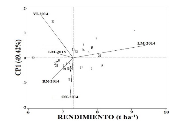
Figure 1 AMMI biplot with the first main component (CP1) and the average yield of 25 hard yellow corn hybrids evaluated in five environments of Peru during the period 2014-2015.
According to the average of the genotypes in the five environments, the national average of 4.5 t ha-1 doubled, according to figures from SIEA (2014). While the five genotypes with lower average yield were the following, in descending order: POOL25xHPM302, CML359xHPM302, CML358xHPM302, EXP-05 and HPM302, having the averages 66.842, 6.84, 6.768, 6.74, 6.151 t ha-1, respectively, of the which, the first three were trilinear hybrids, followed by the double hybrid EXP-05 and finally the genotype HPM302, material used as a female tester with lines and pool of CIMMYT, the latter being the most stable of all genotypes (|≤| al CP1) according to Figure 1; that is, it was the genotype closest to the abscissa axis, which indicates that it was less influenced by the IG*A, as mentioned by Alejos et al. (2006), Palemon-Alberto et al. (2012) and Lopez-Morales et al. (2017) in their respective jobs, HPM302 also being the lowest performer.
Likewise, the four genotypes followed by the most stable, ascending were the following: CML229xHPM302, POOL26xHPM302 (in penultimate place of the genotypes with respect to the highest yield and with a difference of 0.073 t ha-1), CML359xHPM302 (in fifth place, of the genotypes with respect to the lowest yield) and POOL22xHPM302; being these five genotypes those that maintained their behavior through the environments.
On the other hand, the genotype furthest from the abscissa axis was the EXP-05 (double hybrid), which indicates that it had a high IG*A between the environment. Followed by the four less stable genotypes (|≥| al CP1); that is, the genotypes furthest from the abscissa axis, in descending order were: CML225xHPM302, CML453xHPM302 (in third place of the genotypes with respect to the highest yield, with a difference of 0.175 t ha-1), POOL34xHPM302 and POOL33xHPM302 (in fourth place, of the genotypes with respect to the one of greater yield and with a difference of 0.284 t ha-1). Both Table 3 and Figure 1 indicate that the trilinear hybrids POOL26xHPM302 and CML226xHPM302 expressed their maximum potential of average yield, 8.08 and 8.153 t ha-1, respectively, as well as a good stability between environments (|0.5| < CP1).
Between the genotype CML226xHPM302 hybrid trilinear and HPM302 simple hybrid (the genotype of higher and lower yield, respectively) there was a difference of 24.56%, which can mean the difference between seeding trilinear hybrid genotypes and the simple hybrid. In general, all twenty-five genotypes evaluated exceeded the national average of the yield that was 4.5 t ha-1 (SIEA, 2014); meanwhile, only 10 of the 25 genotypes surpassed the general average that was 7.305 t ha-1 (used as coordination axis in Figure 1), leaving among them the double-cross commercial hybrid PM-213 material.
In Figure 1, no material discriminated between environments, indicating that no genotype was superior to the five test environments. At the same time, Figure 1 reports that the HPM302 (simple hybrid) was the most stable of the genotypes (closest to the abscissa) but had the lowest yield among genotypes (6.151 t ha-1). Two commercial double cross hybrids (PM-213 and EXP-05) showed a higher yield (7.613 and 6.740 t ha-1, respectively) with respect to the genotype HPM302 (simple hybrid), but had a higher IG*A, being the EXP-05 is the least stable (the furthest away from the abscissa) between genotypes, as shown in Table 3 and Figure 1.
Meanwhile, the trilinear hybrids ranged from a regular grain yield (CML358xHPM302 with 6.768 t ha-1) to excellent (CML226xHPM302 with 8.153 t ha-1, the highest yield among genotypes) and intermediate stability (|0.5| < CP1) except for the CML453xHPM302, POOL34xHPM302 and CML225xHPM302 genotypes, which are furthest from the abscissa axis; that is, they were more influenced by the IG*A among trilinear hybrids. On the other hand, all the trilinear hybrids evaluated had higher yield than the simple hybrid (HPM302 with 6.151 t ha-1) and only five genotypes of the trilinear hybrids (the highest yielding ones) surpassed the best double cross hybrid (PM-213 with 7.613 t ha-1) by 6.63% with respect to the best trilinear hybrid yield (CML226xHPM302 with 8.153 t ha-1).
From the foregoing it can be mentioned that the trilinear hybrids had an approvable grain yield before the double hybrids (only five genotypes) and simple hybrid (both the trilinear and double hybrids) and most of these hybrids had an intermediate stability, between which were the two trilinear hybrids (POOL26xHPM302 and CML226xHPM302, obtaining the highest significant differences from the rest of genotypes) with the highest grain yield; through, test environments, as reported by González et al. (2009) with similar materials.
On the other hand, in the town of La Molina for the 2014 agricultural cycle (LM-2014) the genotypes showed the highest average yield among localities (9.424 t ha-1, obtaining the highest significant difference from the rest of localities), such performance average was higher; through, of the genotypes, besides being the only locality that surpassed the average performance (7.305 t ha-1 (used as coordinate axis in Figure 1).
According to the length of the vectors with respect to the mean (standard deviation), the environments that best discriminated the genotypes were LM-2014, Viru (VI-2014), Oxapampa (OX-2014) and Rio Negro (RN-2014); on the other hand, the location of La Molina 2015 (LM-2015), did not discriminate between genotypes; that is, it was the most stable of the environments (|0.5| < CP1), which are closer to the abscissa axis; that is to say, it was the least influenced by the IG*A, this could be due to the fact that it was the locality where the crosses of the simple hybrid, and double and trilinear hybrids were evaluated. Noticing a great difference both in the length and direction of the vectors, as well as in the average yields between 2014 and 2015 in the town of La Molina, which can be interpreted as a response to climate changes, such as indicates Table 1, where there are slight changes in maximum and minimum temperatures, as well as in precipitation, with the location of La Molina being higher in 2014 than in 2015.
This opposition in the length and direction in the vectors, and in the average yields in the same locality could be due to the slight difference of climatic changes, as they were presented in the studies of González et al. (2009); López-Morales et al. (2017) finding a similar result before the same locality evaluated in different years or agricultural cycles of the same year. Likewise, the second most stable environment was LM-2014, which obtained the highest average performance, surpassing the two best trilinear hybrids (POOL26xHPM302 and CML226xHPM302) with 9.424 t ha-1, being also statistically significant different in the Tukey test between environments.
Followed by the OX-2014 environment with an average yield of 7.216 t ha-1 and equally statistically separated. Meanwhile, the environment LM-2015 (the most stable) with 6.844 t ha-1 and RN-2014 with 6.674 t ha-1, obtained the same letters in Tukey, which means that between these two environments there were no statistical differences, while the environment with the lowest performance was VI-2014 (the least stable) with an average yield of 6.374 t ha-1 (Figure 1 and Table 3). The two best trilinear hybrids (POOL26xHPM302 and CML226xHPM302) responded well to the environment of La Molina in 2014 and not to 2015, despite the fact that in this locality all crossings of the evaluated hybrids were carried out.
Which means that each locality had its own particularity: better adaptation (LM-2014) and better stability (LM-2015), but the change in rainfall and temperatures was perhaps the difference between the two locations (Table 1 and Figure 1), as reported by Alejos et al. (2006).
Effect of the two main components
In the second AMMI analysis, Figure 2 presents the biplot where the effects of the first two PCs are dimensioned, which explained 70.47% of the IG*A.
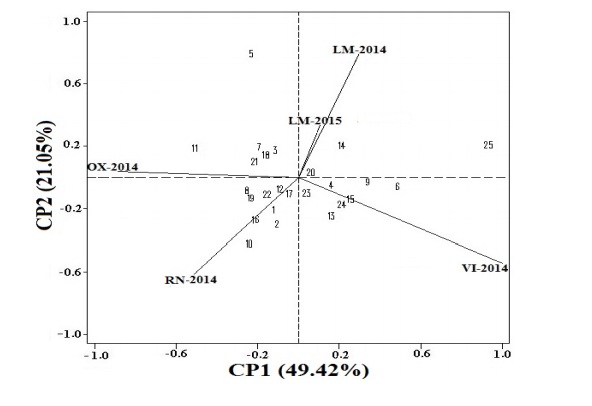
Figure 2 AMMI biplot with the first two main components (CP1 and CP2) of the average yield of 25 hard yellow corn hybrids evaluated in five environments of Peru, during the 2014-2015 period.
In Figure 2, the most stable genotypes or environments are those located at the center of Figure 2 (near the origin), while those farther away at the origin will be more influenced by the IG*A. Thus, in the biplot of Figure 2 it is observed that the most stable genotypes are the following, ordered in descending order to their stability: POOL26xHPM302, CML359xHPM302 and CML229xHPM302 (the three trilinear hybrids) and HPM302 (the only simple hybrid), which coincides with the first four hybrids of Figure 1.
Likewise, they also coincide with the five less stable genotypes (the ones that are farthest from the origin), in ascending order they are the following: EXP-05 (one of the double hybrids), CML228xHPM302, CML453xHPM302, CML225xHPM302 and POOL21xHPM302 (trilinear hybrids), among them only CML228xHPM302 was added in the genotypes which was not in Figure 1 among the least stable, which could be due to the effect of CP2.
Likewise, the LM-2015 environment was the most stable in Figures 1 and 2, while the other four environments evaluated discriminated between genotypes. Yan et al. (2000) indicated that between the vertices of environments with an angle less than 90º will have a similar distribution, which happened between the LM-2014 and LM-2015 environments and also with RN-2014 and OX-2014 (Figure 2). While environments close to 90º, they do not correspond in the way of organizing genotypes, as is the case with RN-2014 and VI-2014, LM-2014 or LM-2015 and VI-2014.
In as much, the atmospheres that are with 180º angles, to order of opposite form to the genotypes, which complicates the selection between these environments for being of different conditions, as it happened between the environments of LM-2014 or LM-2015 and RN-2014. With respect to the genotypes found between angles less than 90º and greater than 270º of each of the vertices of environments, it was the genotypes that expressed their maximum genetic potential in the test environments (Eeuwijk, 2006). Therefore, the vectors of the LM-2014 and LM-2015 environments are too close to each other, which could be due to the edaphological similarity, since it is the same location evaluated in a different year.
Consequently, four groups of genotypes were generated, being the most and least stable in each group, in that order the genotypes were, respectively: for the environment LM-2014 and LM-2015 were genotypes POOL26xHPM302 (the penultimate in highest yield) and CML228xHPM302 (both trilinear hybrids), while in VI-2014 they were POOL26xHPM302 (trilinear hybrids) and EXP-05 (double hybrid and with less stability in Figure 1), while for RN-2014 they were HPM302 (simple hybrid and minor yield) and POOL21xHPM302 (trilinear hybrids) and finally in OX-2014 were the genotypes CML229xHPM302 and CML225xHPM302 (both trilinear hybrids) (Figure 2).
In Figure 2, the vectors of the environments of La Molina (LM-2014 and LM-2015) are very close to each other, although they were evaluated in different years there was no great difference between them, this could happen because they had the same soil conditions (fertilization and soil type) and climatic conditions (precipitation and temperature with less than one difference) (Table 1). The fact that these environments are together, as shown in Figure 2 and fall in the same quadrant means that they are very similar to the IG*A, as indicated in the work of Alejos et al. (2006) where they evaluated different agricultural cycles in the same locality, obtaining similar results of the vectors (length, distance and direction).
However, when plotting CP1 and performance (Figure 1), LM-2014 (with 9.424 t ha-1) was higher than all environments (OX-2014 the second place among environments with 7.216 t ha-1) and genotypes (CML226xHPM302 with the highest yield of 8.153 t ha-1), and even the general average (of 7.307 t ha-1). So Alejos et al. (2006) suggests evaluating in the same place for several cycles in order to be more accurate with the data. The high observed performance of the LM-2014 environment in Table 3 and Figure 1, can be explained by the climatic conditions (precipitation and temperature) are ideal for the cultivation of corn (Table 1), which gave the great advantage not only before the LM-2015 environment, but also to the environments established in other areas of Peru.
The difference in the performance of the LM-2014 locality with the environments of OX-2014 and RN-2014 could have been due to the excess of humidity and a poor distribution of the precipitation, since both locations were rainfed crops where annual rainfall records were obtained with 1 603.4 and 2 466.6 mm, respectively (Table 1). As indicated by Barrales et al. (1984), performance is associated not only with the quantity, but also with the distribution of water. The low yield of the locality of RN-2014 (with 6.674 t ha-1) could also be due to the high temperatures, with a maximum of 33 and a minimum of 25 °C (Table 1), since one of the factors that more affects a plant are high temperatures (>25 °C) (Rincón et al., 2006), because it reduced significantly the yield of grain up to 20.19% with respect to the environment LM-2014 with the highest yield (9.424 t ha-1).
Due to its low dose of fertilization in P and K, as well as its type of soil Arenosol (Table 1), which has the characteristic of high permeability and low capacity to store water and nutrients (IUSS, 2007), in the environment VI-2014 genotypes did not express their maximum genetic potential, which could explain that it was the lowest-yielding locality with 6.374 t ha-1 (Table 3 and Figure 1). Meanwhile, in Figure 2 the vectors (length, distance and direction) of the environments of La Molina (LM-2014 and LM-2015), are very close to each other, being in quadrant I where there is an adaptation and stability positive of the genotypes, which may be due to the fact that it was the locality where all the crossings of the evaluated hybrids (trilinear, double and simple) occurred, which could also generate that the two environments were united, given that the genotypes acted in a very similar way, since it was in the same environment evaluated in different years (2014 and 2015).
Meanwhile, the Leptisol soil of the La Molina environments (Table 1) favored humidity due to its fine texture; that is, they were clay soils that retained higher humidity (IUSS, 2007) under irrigation conditions.
Conclusions
The AMMI model (additive main effects and multiplicative interactions) was a useful tool to interpret the interaction genotype by environment (IG*A) represented in its two biplot graphs, in the characteristic of grain yield and to be able to accurately determine the stability and adaptation of the genotypes evaluated. The biplot graphs of the AMMI model explained 49.42% and 70.47% of the IG*A, respectively. The trilinear hybrids CML226xHPM302 with 8.153 and POOL26xHPM302 with 8.08 t ha-1, presented the best adaptation (yield), standing out statistically from the rest of the genotypes.
Likewise, but in a contrary way, the simple hybrid HPM302 had the lowest performance with 6.151 t ha-1, being among the first places of the genotypes with greater stability, being surpassed by CML226xHPM302 (the first place in performance). While the two double-cross hybrids can be considered superior in grain yield to the simple hybrid but less than six trilinear hybrids. Between the two locations of La Molina evaluated in different years (LM-2014 and LM-2015), there were no soil differences (fertilization and soil type), but there was a slight climatic inequality (precipitation and temperatures).
Therefore, it is inferred that it caused significant effects in each environment: LM-2015 did not discriminate between environments and genotypes, considering the most stable environment, with an average yield of 6.844 t ha-1, LM-2014 discriminated between genotypes, obtaining a maximum average yield potential of the genotypes (9.424 t ha-1), being the only one that exceeded the general average, with the main components of the IG*A positive. Finally, it can be seen that in the biplot charts the best genotypes were the POOL26xHPM302 and the CML226xHPM302 (both trilinear hybrids), since they expressed their maximum potential for yield and stability in the environments of La Molina where edaphoclimatic conditions were suitable for these genotypes.
Literatura citada
Alejos, G.; Monasterio, P. y Rea, R. 2006. Análisis de la interacción genotipo-ambiente para rendimiento de maíz en la región maicera del estado Yaracuy, Venezuela. Agron. Trop. 56(3):369-384. [ Links ]
Barrales, D. S.; Muñoz, O. A. y Sotres, R. D. 1984. Relaciones termopluviométricas en familias de maíz bajo condiciones de temporal. Agrociencia. 58:127-139. [ Links ]
Castillo, D.; Matus, I.; Del Pozo, A.; Madariaga, R. and Mellado, M. 2012. Adaptability and genotype × environment interaction of spring wheat cultivars in Chile using regression analysis, AMMI, and SREG. Chilean J. Agric. Res. 72(2):167-174. [ Links ]
Crossa, J. 1990. Statistical analysis of multilocation trials. Adv. Agron. 44:55-85. [ Links ]
DGCA. 2012. Dirección General de Competitividad Agraria. Cadena agroproductiva del maíz amarillo duro. Ministerio de Agricultura. Lima, Perú. 30 p. http://agroaldia.minagri.gob.pe/biblioteca/download/pdf/agroeconomia/agroeconomiamaizamarillo2.pdf. [ Links ]
Eeuwijk, van F. A. 2006. Genotype by environment interaction. Basics and beyond. In: Plant breeding: The Arnell Hallauer International Symposium. (Eds.). Eeuwijk, van F. A.; Lamkey, K. R. and Lee, M. Blackwell Publishing, Ames, Iowa, USA. 155-170 pp. [ Links ]
Falconer, D. S. 1981. Introduction to quantitative genetics. Longman group limited (2da edition). London. 133 p. [ Links ]
Gauch, H. G. 2006. Statistical analyses of yield trials by AMMI and GGE. Crop Sci. 46:1488-1500. [ Links ]
Gauch, H. G. and Zobel, R. W. 1989. Accuracy and selection success in yield trial analyses. Theor. Appl. Gen. 77:473-481. [ Links ]
González, H. A.; Sahagún, C. J.; Vázquez, G. L. M.; Rodríguez, P. J. E.; Pérez, L. D. de J.; Domínguez, L. A.; Franco, M. O. y Balbuena, M. A. 2009. Identificación de variedades de maíz sobresalientes considerando el modelo AMMI y los índices de Eskridge. Agric. Téc. Méx. 35(2):189-200. [ Links ]
IUSS. 2007. International Union of Soil Sciences. Grupo de trabajo WRB. Base referencial mundial del recurso suelo. Primera actualización. Informes sobre recursos mundiales de suelos No. 103. FAO, Roma, 117 p. http://www.fao.org/3/a-a0510s.pdf. [ Links ]
López-Morales, F.; Vázquez-Carrillo, M. G.; Molina-Galán, J. D.; García-Zavala, J. J.; Corona-Torres, T.; Cruz-Izquierdo, S.; López-Romero, G.; Reyes-López, D. y Esquivel-Esquivel, G. 2017. Interacción genotipo-ambiente, estabilidad del rendimiento y calidad de grano en maíz Tuxpeño. Rev. Mex. Cienc. Agríc. 8(5):1035-1050. [ Links ]
Manrique, C. P. A. 1997. El maíz en el Perú. Consejo Nacional de Ciencia y Tecnología (CONCYTEC). Lima, Perú. 362 p. [ Links ]
Martínez, G. A. 1988. Diseños experimentales. Métodos y elementos de teoría. Trillas. México, DF. 756 p. [ Links ]
Medina, S.; Marín, R. C.; Segovia, V.; Bejarano, A.; Venero, Z.; Ascanio, R. y Meléndez, E. 2002. Evaluación de la estabilidad del rendimiento de variedades de maíz en siete localidades de Venezuela. Agron. Trop. 52(3):255-275. [ Links ]
Palemón-Alberto, F.; Gómez-Montiel, N. O.; Castillo-González, F.; Ramírez-Vallejo, P.; Molina-Galán, J. D. y Miranda-Colín, S. 2012. Estabilidad de cruzas intervarietales de maíz (Zea mays L.) para la región semicálida de Guerrero. Agrociencia. 46(2):133-145. [ Links ]
Paliwal, P. R.; Granados, G.; Renée, L. H.; Violic, D. A. 2001. El maíz en los trópicos: mejoramiento y producción. Organización de las Naciones Unidas para la Agricultura y la Alimentación (FAO). Roma, Italia. 367 p. [ Links ]
Polanco, J. A. y Flores, M. T. 2008. Bases para una política de I&D e innovación de la cadena de valor del maíz. Foro Consultivo Científico y Tecnológico. México, DF. 244 p. [ Links ]
Rincón, T. J. A.; Castro, N. S.; López, S. J. A.; Huerta, A. J.; Trejo, L. C.; Briones, E. F. 2006. Temperatura alta y estrés hídrico durante la floración en poblaciones de maíz tropical. Bot. Exp. 75:31-40. [ Links ]
Samonte, S. O. P.; Wilson, L. T.; McClung, A. M. and Medley, J. C. 2005. Targeting cultivars onto rice growing environments using AMMI and SREG GGE biplot analyses. Crop Sci. 45:2414-2424. [ Links ]
SAS. 2002. Statistical Analysis System. The SAS System for Windows 9.0. User’s guide. Cary, N. C. USA. 584 p. [ Links ]
SENAMHI. 2016. Servicio Nacional de Meteorología e Hidrología del Perú. Mapa climático nacional. Ministerio del ambiente. https://www.senamhi.gob.pe/?&p=mapa-climatico-del-peru. [ Links ]
SIEA. 2014. Sistema Integrado de Estadística Agrarias. Ministerio de Agricultura y Riego (MINAGRI), Perú. Anuario comercial exterior 2014. http://siea.minagri.gob.pe/siea/. [ Links ]
Torres, F. J. L.; Morales, R. E. J.; González, H. A.; Laguna, C. A. y Córdova, O. H. 2011. Respuesta de híbridos trilineales y probadores de maíz en valles altos del centro de México. Rev. Mex. Cienc. Agríc. 2(6):829-844. [ Links ]
Valladolid, R. J. 2003. Crianza ritual de la diversidad de maíces en los Andes del Perú. In: Esteva, G. y Marielle, C. (Eds.). Sin maíz no hay país. CONACULTA. Museo Nacional de las Culturas Populares. México. 67-82 pp. [ Links ]
Vázquez, C. M. G.; Santiago, R. D.; Salinas, M. Y.; Rojas, M. I.; Arellano, V. J. L.; Velázquez, C. G. A. y Espinosa, C. A. 2012. Interacción genotipo-ambiente del rendimiento y calidad de grano y tortilla de híbridos de maíz en valles altos de Tlaxcala, México. Rev. Fitotec. Mex. 35(3):229-237. [ Links ]
Yan, W. and Rajcan, I. 2002. Biplot analysis of test sites and trait relations of soybean in Ontario. Crop Sci. 42(1):11-20. [ Links ]
Yan, W.; Hunt, L. A.; Sheng, Q. and Szlavnics, Z. 2000. Cultivar evaluation and mega-environment investigation based on GGE biplot. Crop Sci. 40:597-605. [ Links ]
Zobel, R. W.; Wright, M. J. and Gauch, H. G. 1988. Statistical analysis of a yield trial. Agron. J. 80:388-393. [ Links ]
Received: March 01, 2019; Accepted: June 01, 2019
 Este es un artículo publicado en acceso abierto bajo una licencia
Creative Commons
Este es un artículo publicado en acceso abierto bajo una licencia
Creative Commons
