Introduction

The production of food in the world satisfies a wide range of functions of vital importance for the welfare of humanity. Besides generating the world’s food, they are also indispensable as a means of subsistence for billions of people as a generator of employment, income and for contributing to rural and general development (^{OECD-FAO, 2016}).

Among them, fruit production stands out, which from 2005 to 2014 had an annual increase in exports of 8.8% and imports of 8.2%. Therefore, fruit trade has practically doubled in the last ten years, with the most important being bananas, grapes and apples (^{SIECA, 2016}).

The fruits of temperate climate constitute one of the most important sources of income of this type of regions since they are more labor-intensive and, therefore, are a greater source of employment. These crops occupy the first place in cultivated area and the second place in the total value of total agricultural production in Mexico (^{Smith and Somerset, 2003}).

On the other hand, the apple in Mexico is one of the five most consumed fruits nationwide with a consumption of 9 kg per year per inhabitant. Its consumption in the country is around 1 000 000 tonnes (t) of which imports 200 000 t. The main national producers are: Chihuahua, whose planted area is 43% of the national surface, Durango 18%, Puebla 14% and Coahuila 12%. Imports come mostly from the United States of America, occupying 94% of them and 5% for Chile (^{SAGARPA, 2015}).

Therefore, the predictive models in the activity of the apple can benefit the producers, packers and buyers, since it can improve the efficiency in making both market decisions and production planning (^{Logan et al., 2016}).

In this sense, for the understanding of a market, it is important to consider the response of prices to changes in supply and demand, as evidenced by the work of ^{Ahrens et al. (2014)}, as well as the importance of price behavior, since for business cycles, for example, it is an important factor in decision making. Also, an inertia in prices comes to cause shocks (unpredictable unexpected event that affects an economy, positively or negatively) permanent demand or supply (^{Noussair et al., 2015}).

To acquire information, economic agents, conceptualize it and take it into account for future decisions, especially prices, it is also pointed out that small price variations can be taken by agents without further analysis, unlike larger variations, where the opposite happens and the decision has to be deliberated (^{Spears, 2014}).

Markets and prices are the central scenario in economic theory, especially its operation and training; however, they are not easy to model, therefore, frequently, the price analysis is aimed at describing the dynamics of the market, although they can be described based on some static analysis or comparative statics (^{Flam and Godal, 2008}).

In this regard, the components of the price that are typically considered in international economy are the production cost, mark ups (value that the economic agent adds to the cost of production) and transaction costs where it is indicated that the cost of production and mark ups they are the main source of price variation (^{Yilmazkuday, 2014}), although one should be aware that economic agents are not always perfectly informed about prices (^{Chudik, 2012}).

The information contained in the market prices is fundamental to the assumption that a market of price takers is being dealt with. Therefore, the efficiency with which market information is processed is important (^{Nelson, 1995}). It becomes necessary, the construction of a useful model, which serves to carry out price predictions (^{Shah and Ghonasgi, 2016}).

The monitoring of prices is important within the budget process, helping to establish objectives, in a regional and national framework, it is essential to establish a price tracking system. The objective of this work was to analyze the price of the apple in order to provide information to the main economic agents of this sector, with a prediction based on a Sarima model that serves as a guide for decision making.

It should be mentioned that this type of model is based on quality data that facilitate its estimation and evaluation in statistical packages (^{Jose and Sojan, 2013}). For the purposes, price will be understood as the amount of money paid in a transaction (^{Fetter, 2016}). But the concept is more than that, given that prices have a decisive influence on the market economy (^{Van Dalen and Thurik, 1998}). For example, one can speak of price policy as one of the main factors for competing in the world market (^{Van Dalen and Thurik, 1998}).

Materials and methods

For the analysis, the price series of the red delicious apple (Malus domestic) was used on a monthly basis, published by the national information and market integration system (SNIIM) on its website. Data were taken from January 1998 to July 2017 with a total of 235 observations which were analyzed with the GRETL^® software.

Taking into account that a time series is a succession of observations of a variable measured at regular intervals of time, its analysis objective being to know the behavior of said variable; through time, to be able to make predictions about it, clarifying uncertainty for economic agents (^{Parra, 2011}).

To complete the objective, a univariate analysis of time series was applied, that is, they use the same information contained in the previous values of the series. In this regard, it should be borne in mind that a time series consists of trend, cyclical fluctuation, seasonal variation and irregular movements or error; however, in a specific series, the four components do not have to be given (^{Parra, 2011}).

Within the previous foundations for its quantification, it is worth noting that in 1970, Box and Jenkins developed a methodological body destined to identify, estimate and diagnose dynamic models of time series in which the time variable plays a fundamental role (Arce, 2010). Concepts that have become later in the integrated autoregressive models of moving averages (ARIMA).

In this context, a model is defined as autoregressive if the endogenous variable of a period t is explained by observations of itself corresponding to previous periods, adding, as in structural models, an error term. In the case of stationary processes with normal distribution, the statistical theory of stochastic processes says that, under certain preconditions, all Yt can be expressed as a linear combination of its past values plus an error term (Arce, 2010).

One of the most frequent approaches to manage seasonality in the time series has been to calculate it using a seasonal decomposition procedure, since the analysis of its predictions shows a higher precision, indicating that an estimate is more efficient combining the seasonal component than with a single individual pattern. However, there seems to be no consensus on which model is preferable to use for this type of analysis and prediction (^{De Gooijer and Hyndman, 2006}).

For its quantification, it is assumed that the series can be represented by Yt= 1, … ,T being Yt a monthly random variable that follows a SARIMA model (p,d,q)(P,D,Q)12 , in such a way that we proceed to identify and estimate the model, which generally is:

Where: L = is the delay operator; μ= is the mean of the differentiated series, ϕL , θ(L) , ΦL12 and Θ(L12) are polynomials of order p, q, P and Q respectively, with the short-term dynamics collected by the first two and the seasonal dynamics by the last two, ϕL and ΦL12 forming the autoregressive part of the model, while θ(L) and Θ(L12) make up the moving average. Δd= (1-L)dandΔD= (1-L12)D , where d= is the order of integration and D= is the order of seasonal integration. Finally, we assume that εt = is a white noise with Gaussian distribution i. i. d. N(0, σε2) .

Results and discussion

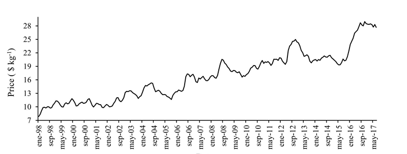
In the time series of the price of the apple from January 1998 to July 2017, a variance was noticed that is increasing; that is, the oscillation within a year is getting bigger and bigger. To minimize this variance, the series was transformed into logarithms (Figure 1).

Figure 1 Price of the apple. Elaboration with SNIIM data.  

In Figure 2, after having converted the series to logarithms, a reduction in variance was analyzed.

Figure 2 Logarithm of the price of the apple. Elaboration with SNIIM data.  

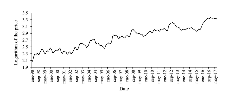
According to the methodology of ^{Box and Jenkins (1970)}, the series of logarithms must be transformed into first differences, since we intend to work with a stationary series in variance and trend. For the series to be stationary in trend, then the first difference is applied.

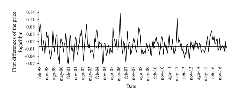
In Figure 3, in first differences, it is perceived that the series oscillates around 0, no longer has a tendency and its variance is more or less constant. But, a seasonal component is detected, therefore, a transformation is made at 12 months or seasonal difference.

Figure 3 First differences of the logarithm of the price of the apple. Elaboration with SNIIM data.  

In the Figure 4 shows the first regular and seasonal difference, from this transformation is where we work. The correlogram is obtained to identify the type of pattern it contains.

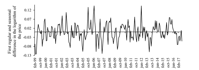
Figure 4 First regular and seasonal difference of the series in logarithms of the apple. Elaboration with SNIIM data.  

The Dickey-Fuller unit root test was applied in Table 1, where it was perceived that, given the null hypothesis that the series has a unit root is rejected, it is concluded that it is a seasonal series.

The correlogram of Figure 5 was analyzed, in order to determine the type of model that best suits the series in the simple and partial autocorrelation functions, it was observed that it can be an autoregressive model of order 2 in the regular part and in the seasonal part of an autoregressive of order 1, being able to be identified as a typical process of an economic series according to ^{Arce (2011)}.

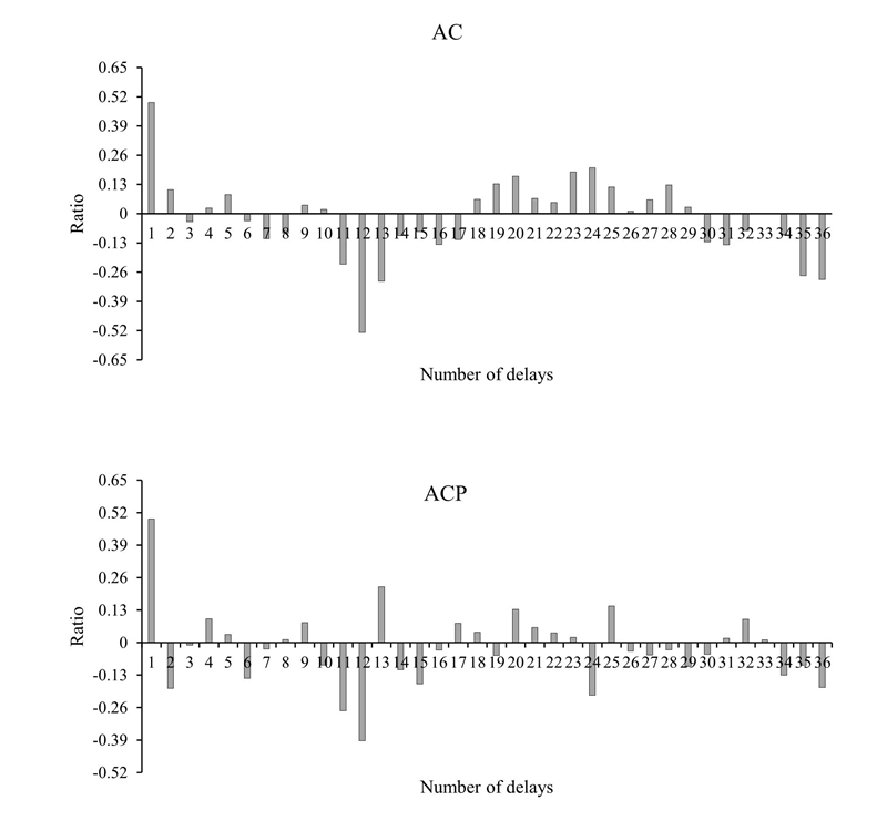
Figure 5 Correlogram of the first regular and seasonal difference of the series in logarithms of the apple price. Results obtained in Gretl^® and edited in Excel.  

Then we select an ARIMA2, 1, 0×ARIMA(1, 1, 0)12 model over the series in logarithms of the price. The model is run in Gretl^® to obtain the results of Table 2, which highlights that both the regular and seasonal part are significant. It should be noted that Gretl^® calculates by the maximum likelihood method.

The result is presented in the following equation:

It is proceeded to verify that the contrast of normality of waste actually passes as it is distinguished in Figure 6 and in fact, it was found that the errors are distributed normally.

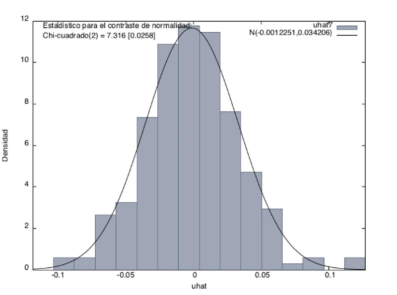
Figure 6 Contrast of normality of the errors of the Sarima model of the price in logarithms of the apple. Source: results obtained in Gretl^®.  

The contrast of the correlogram or correlogram of the residues was made in Figure 7, where it was verified that we are indeed in the presence of white noise. It is reaffirmed that it is before an ARIMA2, 1, 0×ARIMA(1, 1, 0)12 model.

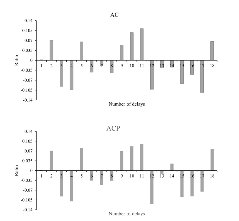
Figure 7 Correlogram of the residuals of the Sarima model of the price in logarithms of the apple. Results obtained in Gretl^® and edited in Excel.  

It is proceeded to make a forecast, which will be for one year before the last data; that is, 12 observations forward in time. As expected, as the value moves away in time, the confidence interval increases as it is perceived in Figure 8, where it only shows 100 observations.

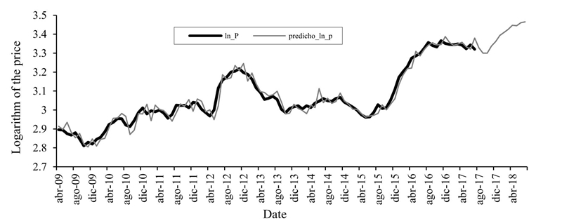
Figure 8 Prediction of the Sarima model of the logarithm price of the apple for one year. Results obtained in Gretl^® and edited in Excel.  

Thus, the prediction of the price for the following months would be represented by Table 3, where the real price is also compared against its predicted and the relative error is calculated from July 2015 to July 2017, with the relative error being around 2%, which indicates that the prediction of the model can be relatively good. This prediction does not indicate an upward price trend until the end of the same in July 2018. Following the forecast generates a price of $31.99 for the month of July 2018, which is an increase of 4 pesos with respect to July 2017.

From the results obtained, it means that the estimated model represents a good statistical adjustment of the time series of the price of the apple, given that a relative error of only 2% is handled when in Wei et al. (2010) a relative error of 5% is accepted. Regarding the identification of the model ^{Caivano et al. (2016)}, indicates that with seasonal series a double or triple interaction are sufficient, to adjust it.

Unlike Yoonsuk and Wade (2016), the model was adjusted without the correction of outliers. However, as anticipated by ^{Findley et al. (2016)}, with a difference in the seasonal part is enough to adjust the model. However, despite the fact that the use of this type of models has increased in recent years, the opinion persists that there is no consensus on which type of model is the one that best fits the economic data that present seasonality (^{Franses and Van Dijk, 2005}).

Comparing with the ARIMA methodology, sugar production prediction works in Mexico have models with an accuracy in the forecast of 94%, such as that of Ruiz et al. (2011), which has an ARIMA structure (1, 2, 0).

Other production prediction models, that contemplate both ARMA structures, such as ARIMA, are those presented for the production of milk and the production of pork. In the works of Sánchez et al. (2013) and ^{Barreras et al. (2013)} in which it is accepted that they are useful to establish only short-term forecasts, suggesting the use of multivariate models for a longer term.

^{Martínez and Chalita (2011)} use an ARIMA model (23, 0, 1) to make a 12-month forecast on the tomato price, where they conclude that the current and future prices of the vegetable can be explained by their past prices.

In any case, the presentation of a unique and universally accepted model is unreal and possibly unnecessary. The important thing is that the model is well specified, so that it is well understood and analyzed, coinciding with the structure of the series (^{Maravall, 1993}).

Finally, as ^{Franses and Van Dijk (2005)} warn, simple seasonal models offer a better prediction in the short term, while more elaborate models can serve to predict in the long term.

Conclusions

Through the analysis of the time series of the red delicious apple price, from January 1998 to February 2017, a Sarima ARIMA2, 1, 0×ARIMA(1, 1, 0)12 model was established, in which since the errors are distributed in a normal way; that is, it is in the presence of white noise. The adjustment of the results of the model was obtained in a convincing and practical way in the Gretl^® software. In addition, apple prices were forecast for the months of August 2017 to July 2018, where it should be noted the trend to rise them, with a relative error around 2%, which is close to ideal. However, one must be aware of the limitation of the prediction, since they are predicted values and the economic dynamics ergo that of prices will always be complex.