Study area

The state of Aguascalientes is 22° 27' and 21° 38' north latitude, 101° 53' and 102° 52' west longitude; and it has a land area of 5 680.33 km2; neighboring to the north, northeast and west with Zacatecas and south and east with Jalisco (^{INEGI, 1995}). The state has three types of climate: temperate semi-dry (BS₁k), semi-dry warm (BS₁h) and temperate sub-humid with summer rains C (w). In such climates the average annual temperature is 17.1, 20.1 and 14.5 °C, respectively; and average precipitation of 488, 579.1 and 688.3 mm respectively (^{Garcia, 1973}; ^{INEGI, 2013}).

Weather information

Daily data of T_max and T_min from traditional weather stations in the state of Aguascalientes were used, these stations belong to the National Weather Service (SMN) (Table 1). For T_max the information available from 56 stations was used, while for T_min the information available in 51 stations.

Table 1 Weather Stations used in the study. 

With daily data of T_max and T_min of each month, the monthly average for each station was obtained, the monthly average was the one used in the trends analysis. For T_max it counted with 672 time series; i.e. 56 stations by 12 months; for T_min 612 time series were obtained; i.e. stations 51 by 12 months.

Mann-Kendall test

The Mann-Kendall test is a nonparametric statistical technique that evaluates the significance of a trend. The test uses the Mann-Kendall statistic which is obtained with (^{Hamed, 2008}):

Where: x_j and x_k represent the variable in years j and k, and also j> k.

Then S variance is given by:

Where: g is the number of consolidated groups and tp is the number of data in the pth group.

Then with S and VAR (S) the statistic test is estimated:

A positive value for Z indicates upward trend, while a negative value indicates a downward trend. H0 is rejected in favor of HA if the absolute value of Z is greater than Z_1-α/2 (^{Hamed, 2008}); the value of α used in this study was 0.05.

After the hypothesis test, the change rate of the variable is calculated with (^{Theil, 1950}):

Where: x_i' and x_i are the data values in the times i' and i, also i'> i. Then it makes N' the number of data where i'> i. Median of N' values of Q is Sen slope or the change rate of the variable (^{Sen, 1968}).

Minimum temperature

Table 2 shows the most outstanding parameters from the trend analysis of T_min. Of the total (612) series of T_min studied, 365 (59. 64%) series showed no statistically significant trend, the remaining 247 (40.36%) series had a statistically significant trend (p≤ 0.05). Of Series with statistical significance, 129 (21.08%) had positive trend and 118 (19.28%) had negative trend.

Table 2 Summary of time series and trends (°C decade-1) for minimum temperature in Aguascalientes. 

T= total, (%) = porcentaje; NO SIG= series con tendencia no significativa; SIG = series con tendencia significativa, SIG+= series con tendencia positiva significativa; SIG- = series con tendencia negativa significativa, MAX + = tendencia positiva significativa máxima; MIN += tendencia positiva significativa mínima; MEDIA+= tendencia positiva significativa media; MAX-= tendencia negativa significativa máxima; MIN-= tendencia negativa significativa mínima y MEDIA- = tendencia negativa significativa media.

The positive trends are present in the twelve months of the year, but most of them concentrated in February and from April to October (Table 2). The month with the highest positive trend was April with 1.33 °C decade^-1 in the station Los Negritos, meanwhile the lowest positive trend occurred in July and September with 0.09 °C decade^-1 in the station Presa Plutarco Elias Calles. The average of significant positive trends for the 12 months was 0.50 °C decade^-1; this value is similar to the average (0.496 °C decade^-1) that ^{Santillan et al. (2011)} reported for the neighboring state of Zacatecas. There is also similarity with the average trend reported by ^{Al Buhairi (2010)} (0.50 °C decade^-1) for the semi-arid City of Taiz, Republic of Yemen, and Al-Hadhrami and ^{Rehman (2012)} (0.508 °C decade^-1) for Saudi Arabia; besides the average positive trend of each month varied between 0.43 and 0.57 °C decade^-1 for January and October, respectively.

Negative trends are also present in the twelve months of the year, but most of them concentrated in January, from April to September and December (Table 2). The month with the highest negative trend was December with -1.42 °C decade^-1 in the station El Ocote I, meanwhile the lowest negative trend was in August with -0.14 °C decade^-1 in the station Calvillo. The average of all significant negative trends of the 12 months was -0.59 °C decade^-1; this value is similar to the average (-0.705 °C decade^-1) that ^{Santillan et al. (2011)} reported for the neighboring state of Zacatecas. Meanwhile the average of the negative trends of each month ranged from -0.49 in June and September to -0.81 °C decade^-1 in December.

Maximum temperature

Table 3 shows the most outstanding parameter from the trend analysis in T_max. Of the total (672) series of T_max studied, 448 (66.67%) series had no statistically significant trend, the remaining 224 (33.33%) series had statistically significant trend (p≤ 0.05). Of the total series with significant trend, 167 (24.85%) had positive trend and 57 (8.48%) had negative trend.

Table 3 Summary of time series and trends (°C decade^-1) for maximum temperature in Aguascalientes. 

T= total, (%) = porcentaje; NO SIG= series con tendencia no significativa; SIG = series con tendencia significativa, SIG+= series con tendencia positiva significativa; SIG- = series con tendencia negativa significativa, MAX + = tendencia positiva significativa máxima; MIN += tendencia positiva significativa mínima; MEDIA+= tendencia positiva significativa media; MAX-= tendencia negativa significativa máxima; MIN-= tendencia negativa significativa mínima y MEDIA- = tendencia negativa significativa media.

The months with fewer numbers of positive trends in T_max were in September and November with seven and six series, respectively. The month with the highest positive trend was April with 1.59 °C decade^-1 in the station La Tinaja II, while the lowest positive trend was in December with 0.18 °C decade^-1 in the station Presa Plutarco Elias Calles. The average positive trend during the 12 months was 0.61 °C decade^-1; this value is similar to the average (0.79 °C decade^-1) that ^{Santillan et al. (2011)} report for the neighboring state of Zacatecas. Our average positive trend is slightly below to average (0.86 °C decade^-1) of positive trends cited by Al-Hadhrami and ^{Rehman (2012)} for Saudi Arabia. The monthly average of the positive trend in maximum temperature was between 0.37 and 0.82 °C decade^-1 in November and April, respectively.

Arelatively small proportion (57) of series with negative trends in T_max was obtained. The month with the highest negative trend was October with -1.51 °C decade^-1 in the station in San Francisco de los Romo, meanwhile the less negative trend was in September with -0.19 °C decade^-1 in the station Campo Experimental Pavbellón. The average signif icant negative trend during the 12 months was -0.68 °C decade^-1. The average value of the negative trend of T_max was similar to that reported (0.648 °C decade^-1) by ^{Santillan et al. (2011)} for the state of Zacatecas. Moreover, the average monthly negative trend ranged between -0.38 and -0.86 °C decade^-1 in May and October respectively.

The sum of the series with positive trends in T_max and T_min resulted in a total of 296, while the sum of series with negative trends in both temperatures produced a total of 175; this gives an idea that in Aguascalientes there is an upward condition to warming than to cooling which agrees with the situation prevailing in Zacatecas (^{Santillán et al., 2011}) and in other regions of Mexico (^{Pavia et al., 2009}).

Origin of temperature changes

There are different arguments associated to change in temperature patterns. Some reasons are the increased cloud cover, changes in evaporation and precipitation patterns, direct absorption of the infrared portion of the incoming solar radiation, the presence of aerosols, chemical reactions of atmospheric water vapor and increased soil moisture (^{Henderson, 1992}; ^{Hansen, 1995}). ^{McNider et al. (1995)} comment that other cause could be the change in surface roughness due to the onset of trees or establishment of buildings, this alteration of roughness leads to warmer temperatures due to reduced wind speed. In the 1980's there was already evidence that some regions of Aguascalientes had significant reduction in forest area and the appearance of shrubs, these changes in vegetation coincided with the period of increase in the average temperature of 0.4 °C (^{Lemus and Gay, 1988}).

Environmental effects of temperature changes

According to ^{Santillán et al. (2011)} when T_max and T_min trends are analyzed there are nine possibilities: 1) T_max and T_min stable; 2) T_max stable and negative trend of T_min; 3) T_max stable and positive trend of T_min; 4) negative trend of T_max and T_min stable; 5) Positive trend of T_max and T_min stable; 6) negative trend of T_max and T_min; 7) positive trend in T_max and T_min; 8) negative trend in T_max and positive trend in T_min; and 9) positive trend in T_max and negative trend in T_min. When the possibilities two, five and nine are present; there is an increase of RTD by increasing RTD, it increases the evaporation capacity of the atmosphere, the relative humidity decreases, increases crop reference evapotranspiration (ETO), increases the actual crop evapotranspiration (ETC) and increases the irrigation water volume required (^{Tabari et al., 2011}; ^{Xiaomang et al., 2011}). When the possibilities three, four and eight are present; there is a reduction in RTD by reducing RTD, decreases the evaporation capacity of the atmosphere, the relative humidity increases, decreases crop reference evapotranspiration (ETO), decreases the actual crop evapotranspiration (ETC) and decreases irrigation water volume required. When possibilities six and seven are present could be an increase or decrease in RTD, this will depend on the change rate of each of the temperatures.

Table 4 shows the nine possible cases of T_max and T_min obtained for Aguascalientes; the month column appears the number of stations present for each case. It is appreciated that case one had the greatest number of stations (237). Note that adding stations involved in cases 5, 2 and 9, 180 stations are obtained, all of them show the condition of increased RTD. Moreover, if the stations involved in cases 3, 4 and 8 are added, 110 stations are obtained and all of them show the condition of reduced RTD. It is important to add that cases 7 and 6 could also have modifications of RTD as trend lines are not quite parallel, i.e. differ in the change rate, for these cases 67 stations are involved.

Table 4 Trend cases of maximum and minimum temperature and number of stations per month. 

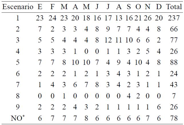
*Se refiere al número de estaciones en cada mes que no contaron con temperatura mínima.

Finally, Figure 1 shows examples of time series for T_max, T_min and RTD in the station Sandovales. For T_max case there was a significant trend for six months (February to June and December), while the trend in T_min was significant for eight months (April to November). Consequently, RTD showed significant trend in 11 months (February to December), note that in those months the trend line is positive which gives an idea that the climate of the locality is more extreme and has more deficit of environmental humidity.

Figure 1 Time series for T_max, T_min and RTD from January to December in the station Sandovales