


![Producción natural de huitlacoche [Ustilago maydis (DC) Corda] en el estado de Aguascalientes](/img/pt/next.gif)


Serviços Personalizados
Journal
Artigo
 texto em
  Inglês (pdf)
 Artigo em XML
 Referências do artigo
 Enviar este artigo por email
Indicadores
-
 Citado por SciELO
 -
 Acessos
Links relacionados
-
 Similares em
SciELO
Similares em
SciELO
Compartilhar

 Permalink
Revista mexicana de ciencias agrícolas
versão impressa ISSN 2007-0934
Rev. Mex. Cienc. Agríc vol.7 no.5 Texcoco Jun./Ago. 2016
Articles
Backpropagation artificial neural network versus empirical models for estimating daily global radiation in Sinaloa, Mexico
1Campo Experimental Valle de México-INIFAP. Carretera Los Reyes-Texcoco, Coatlinchán, km 13.5, C. P. 56230, A. P. 307 y 10, Texcoco, Estado de México, México. Tel: 01 800 088 2222, Ext. 85565. (rcervanteso@hotmail.com).
2Universidad Autónoma Chapingo, Departamento de Irrigación, Sección Meteorología agrícola, km 38.5, Carretera México-Texcoco, C. P. 56230, Estado de México, México. Tel: 01 (595) 95 21500. Ext. 5157. (mvazquezp@correo.chapingo.mx).
3Instituto Mexicano de Tecnología del Agua, Paseo Cuauhnáhuac 8532, Colonia Progreso C. P. 62550, Jiutepec, Morelos, México. Tel: 01 (777) 3293 600. Ext: 445. (wojeda@tlaloc.imta.mx).
The results were compared of average daily global radiation model estimated with artificial neural network (RNA) backpropagation against those obtained by empirical models Hargreaves, Angström-Prescott and these calibrated. A model of backpropagation artificial neural network was used with Levenberg Marquardt algorithm for forecasting average daily global radiation four stations located in the irrigation district 075 Valle del Fuerte, Los Mochis Sinaloa, Mexico. The database represents daily averages with 1 484 data vectors for training, validation and test and 229 for prognosis. Among the input variables provided by the irrigation district they were: minimum temperature and maximum temperature, others were calculated as actual duration of sunshine, photoperiod and extraterrestrial solar radiation. The scenarios with one, two and three hidden layers with different numbers of neurons in each hidden layer was obtained. The RNA e6{27} with entries minimum temperature, maximum, hours shine sun divided by photoperiod and extraterrestrial solar radiation, obtained the best fit with a RMSE of 1.6871 and R2 of 0.89 for 1 484 and for data for 229, the AngstromPrescott won the calibrated model with RMSE of 2.2812 and R2 of 0.89. For 1484 average data, the e6{27} scenario presents the best estimate of daily global radiation (Rs) and is better than the empirical models, however for 229 data the Angstrom-Prescott calibrated model provides an estimate of Rs better e6{27} of the RNA.
Keywords: Angström-Prescott; Hargreaves; averages; artificial neural network; solar radiation
Se compararon los resultados de los promedios de radiación global diaria estimados con el modelo de red neuronal artificial (RNA) bakpropagation contra los obtenidos por los modelos empíricos Hargreaves, Angström-Prescott y los calibrados de estos. Se utilizó un modelo de red neuronal artificial backpropagation con el algoritmo Levenberg Marquardt para el pronóstico de los promedios diarios de radiación global de cuatro estaciones ubicadas en el distrito de riego 075 Valle del Fuerte, Los Mochis Sinaloa, México. La base de datos representa promedios diarios con vectores de 1 484 datos para entrenamiento, validación y prueba y 229 para pronóstico. Entre las variables de entrada proporcionadas por el Distrito de riego, fueron: temperatura mínima y temperatura máxima, otras fueron calculadas como: duración real de la insolación, fotoperiodo y radiación solar extraterrestre. Se obtuvieron escenarios con una, dos y tres capas ocultas, con diversos números de neuronas en cada capa oculta. La RNA e6{27} con las entradas temperatura mínima, máxima, horas brillo sol dividida por el fotoperiodo y radiación solar extraterrestre, obtuvo el mejor ajuste, con un RMSE de 1.6871 y R2 de 0.89 para los 1484 datos y para los 229, lo obtuvo el modelo Angström-Prescott calibrado con un RMSE de 2.2812 y R2 de 0.89. Para los 1 484 datos promedios, el escenario 6{27} presenta la mejor estimación de la radiación global diaria (R s ) y es mejor que los modelos empíricos, sin embargo para los 229 datos el modelo Angström-Prescott calibrado presenta una estimación de Rs mejor al e6{27} de la RNA.
Palabras clave: Angström-Prescott; Hargreaves; promedios; radiación solar; red neuronal artificial
Introduction
The daily global radiation is important in areas such as engineering, agriculture, soil physics, agricultural hydrology modeling crops and estimation of evapotranspiration, as well as: modeling climate and weather, growth monitoring crop and disease control.
The radiation reaching the surface of the earth due to gases, clouds and particles in the atmosphere, they absorb and scatter radiation at different wave levels. The need for records of solar radiation becomes important due to the increase in solar energy applications. Obtain reliable data radiation requires systematic measurements (Muribu, 2008).
The artificial neural networks have proven to be excellent tools for different areas of research; since they are able to handle nonlinear relationships (approximation of nonlinear function), separating data (data classification), find hidden relationships in data groups (clustering) or modeling natural systems (simulation) (Demuth et al., 2008)
In estimating global radiation by artificial neural networks is the work of Hasni et al. (2012) cited by Yadav and Chandel (2014) estimated the global radiation each time using an artificial neural network using temperature and relative humidity with a feedforward backpropagation algorithm, similarly Jiang (2008) used an artificial neural network (RNA) of this type to make a prognosis of diffuse solar radiation and compares the results with two empirical models. Rehman and Mohandes (2008) used an artificial neural network model to estimate recurrent global radiation measured temperature and relative humidity values as inputs. Martínez-Romero et al. (2012), used to linear regression models, the model Hargreaves Hargreaves calibrated and RNA to estimate global solar radiation data with average monthly maximum temperature, minimum and extraterrestrial solar radiation. Regarding empirical models Bandyopadhyay et al. (2008), used: Hargreaves, calibration of Angstrom-Prescott and Bristow and Campbell (Bristow and Campbell, 1984) to estimate solar radiation.
The aim of this study was to compare the results of estimates of average daily global radiation four stations, located in the Irrigation District 075, Valle del Fuerte, Los Mochis, Sinaloa, made with the model of artificial neural network (RNA) backpropagation against the estimates obtained by empirical models Hargreaves, Hargreaves calibrated, Angstrom-Prescott and Angström-Prescott calibrated. The averages of the data were used by the proximity of a station to another, since there are no significant differences in climate prevailing between stations.
Materials and methods
Study area and climate data set used
The measured data were used from april 1997 to may 2001 (training, evaluation and validation) and from june to december of the same year (for forecast), maximum temperature, minimum temperature, maximum relative humidity, minimum, and global radiation daily. Subsequently, the averages of all the variables of the four stations, located in 075 DR Valle del Fuerte, in Los Mochis, Sinaloa obtained, whose names (keys), latitudes, longitudes and altitudes are: Ruiz Cortínez (3 843 II-2), 25° 39’ 15”, 108° 45’ 20”, 31 msnm; Batequis (3 546 II-3), 25° 45’ 49”, 32 msnm AC Santa Rosa 1 (3 765 III-1), 25° 45’ 03”, 108° 57’ 21”, 40 msnm; AC Santa Rosa 2 (9 610 III-1) 25° 51’ 16”, 108° 52’ 03”, 61 msnm; and finally: the extraterrestrial solar radiation (Ra), and photoperiod (N), were calculated as the present Allen et al. (1998) and the sun shine hours (n) as recommended by the WMO (1996).
Artificial neural networks
To apply the model of artificial neural networks (RNA) a set of input data is needed, these are divided to: training, validation and testing. The number of hidden layers and the number of neurons in each layer have defined, the activation function is:
Where: x1, x2, …, xm are the input signals; wk1, wk2,…, wkm are the synaptic weights of neuron k; bk is the bias; φ(⋅) is the activation function (Equation 2) and yk is the output signal of the neuron
The algorithm used in this work for the RNA was the feedforward backpropagation, is based on the learning rule error correction, this is a generalization of the algorithm of least square error and consists of two passes through the different layers network, a pass forward and one step back (Haykin, 2008).
The nomenclature to describe a scenario in RNA is expressed as eX{1x2x1}, where eX denotes the stage "X", parentheses key type {1x2x1}, indicate that having 1, 2, and 1 number of neurons in the first , second and third hidden layers, respectively, that is, three hidden layers. The different scenarios with their respective input variables considered for the training of RNA backpropagation below: e1{Tmin, Tmax, Ra}, e2{Tmin, Tmax, n}, e3{n, N, Ra}, e4{Tmin, Tmax, n/N}, e5{Tmin, Tmax, n, Ra}, e6{Tmin, Tmax, n/N, Ra}, e11{n/N, Ra}, e12{Tmax-Tmin, n}, e13{Tmax-Tmin, Ra}, e14{Tmax-Tmin, n, Ra}, e15{Tmax-Tmin, n/N, Ra}. For vectors 1 484 data were used: 25%, 25% and 50% for testing, validation and training, respectively (Demuth et al., 2008).
Empirical models
The Hargreaves equation, according to Allen et al. (1998) and Hargreaves and Samani (1982) is:
Where: Ra is the extraterrestrial radiation [MJ m-2 d-1], Tmax is the maximum air temperature [°C], Tmin is the minimum air temperature [°C], kRs is an adjustment coefficient (0.16 .. 0.19) [°C-0.5], kRs ≈ 0.16 for locations where land mass dominates and air masses are not influenced by a large body of water, and kRs ≈ 0.19 for "coastal" areas. Of Equation 3 the Equation 4 is obtained, with which the calibration is done:
Where: z is the exponent (1/2) renamed, this equation is a linear regression.
The model of Angstrom-Prescott according to Allen et al. (1998) to calculate the solar radiation is:
Where: Rs is solar or shortwave radiation [MJ m-2 d-1], n is the actual duration of sunshine [hours], N is the maximum possible duration of sunshine [hours], n/N is the relative duration of sunshine [dimensionless], Ra is extraterrestrial radiation [MJ m-2 d-1], as is the regression constant, which expresses the fraction of radiation alien who comes to earth on very cloudy days, as + bs is the fraction of extraterrestrial radiation reaching the earth on clear days. Allen et al. (1998) recommend using values as= 0.25 and of bs= 0.50. The Angstrom-Prescott model (Equation 5) was calibrated by a linear transformation coefficients obtained as= -0.5535 and bs= 1.3824 with 1 484 data vectors, the very skewed data were eliminated. The n information not available was estimated according to WMO (1996) and Linacre (1992), who propose yes in one hour has a value greater than 120 W m2, then there is sun shine one hour.
Statistical evaluation
To evaluate the performance (estimate) of the models used the average standard error or square root mean square error (RMSE), the average error (MBE), also called bias or deviation were used, this characterizes the goodness of each models and the coefficient of determination (R2) given by the following equations:
Where: ai is estimated by the model data, ti is the observed data, to ā is the average of the data estimated by the model,
Results and discussion
The model Hargreaves uncalibrated with kRs= 0.19 with 1 484 data obtained an RMSE of 5.6735 and for kRs= 0.16 obtained an RMSE of 3.4062 and the same R2 (0.59) is preserved for 229 data validation found a RMSE of 6.8224 and 3.3696 for kRs 0.19 and 0.16 respectively and R2 of 0.73 for both. The values of z and kRs model Hargreaves calibrated were 0.2995 and 0.2711, respectively, and the estimated values of global radiation for the 1 484 data showed a RMSE of 3.0068 and an R2 of 0.65 and for 229 data validation RMSE of 3.2460 with an R2 of 0.75 for this model. As seen with kRs= 0.16, better fit than a kRs= 0.19, indicating that the irrigation district 075, where the four seasons are located is close to being a locality where land mass dominates according to obtained criteria Allen et al. (1998) and the calibrated model generated better fit the standard error and the coefficient of determination, however, that the kRs the calibrated model is far from 0.16; Martínez-Romero et al. (2012) found RMSE calibration of 1.43 MJ/m2day for Hargreaves model with kRs 0.15928, to estimate monthly average values of global solar radiation, this value kRs say the authors hardly differs from the value of 0.16 so they used the latter for the RMSE of spatial and temporal validation, 1.23 and 1.66 MJ/m2day respectively, against a calibration RMSE of 1.17 MJ/m2day for RNA with entries maximum temperature, minimum and extraterrestrial solar radiation.
The model of Angstrom-Prescott uncalibrated obtained an RMSE data for 1484 5.1948, with an R2 of 0.73 for the calibrated model (as= -0.5535 and bs= 1.3824) the RMSE obtained was 2.0889 with an R2 of 0.84, this indicates that presented better fit the Angström-Prescott model calibrated the calibrated Hargreaves, corroborating indicated in Cervantes-Osornio et al. (2012). Liu et al. (2009) calibrated the coefficients a and b with daily data, finding a better approximation of the global radiation model AngstromPrescott calibrated the calibrated Hargreaves, unlike what was found by Bandyopadhyay et al. (2008), who used the model modified Hargreaves, and Angstrom-Prescott calibrated to estimate monthly solar radiation data and found that the method modified by Hargreaves Annandale et al. (2002) it was better than the Angstrom-Prescott. Almorox et al. (2008) and Meza and Varas (2000), estimated the monthly global radiation with the equation of Angström-Prescott, resulting in this model with the calibrated coefficients is a useful tool, which corroborates the findings in this paper, calibrate models generates a better fit than not.
In the Table 1 shows the results of the average standard error and average error for the training scenario 2, which was one of those who had values of RMSE and MBE closer to zero, in this observed shown that increasing the number of layers hidden not had an impact on improving the fit of RMSE and MBE, as the closest zero adjustment was training with two hidden layers of 24 x 24 neurons in these, in training with a hidden layer the best fit was the one who had 30 neurons in this and three hidden layers was 9 x 24 x 9 neurons, whose best fit of this last block did not exceed the two layers. Additionally, the increased number of neurons in the hidden layers, does not necessarily improve the fit of these tests, for two and three hidden layers, but e2, with a hidden layer obtained the best fit with the maximum number of neurons (30).
Table 1 RMSE and MBE to 1484 data, the stage with 2 inputs: minimum temperature, maximum brightness and sunshine hours.
| 1 capa oculta | e2{Tmin, Tmax, n} 1484 datos | 2 capas ocultas | e2{Tmin, Tmax, n} 1484 datos | 3 capas ocultas | e2{Tmin, Tmax, n} 1484 datos | |||
| RMSE | MBE | RMSE | MBE | RMSE | MBE | |||
| {3} | 1.8121 | -0.0095 | {3x3} | 1.7906 | -0.014233 | {3x3x3} | 1.854 | -0.0092 |
| {6} | 1.7880 | 0.0981 | {6x6} | 1.7877 | 0.0255249 | {3x6x3} | 1.7992 | -0.0169 |
| {9} | 1.7944 | -0.0028 | {9x9} | 1.908 | -0.013783 | {6x9x6} | 1.7974 | 0.0268 |
| {12} | 1.7974 | 0.05675 | {12x12} | 1.7643 | -0.033802 | {6x12x6} | 1.806 | -0.0719 |
| {15} | 1.8884 | 0.1316 | {15x15} | 1.7761 | -0.058406 | {6x15x6} | 1.8573 | -0.0022 |
| {18} | 1.7808 | -0.0835 | {18x18} | 1.7653 | -0.097926 | {9x18x9} | 1.7971 | -0.03131 |
| {21} | 1.7949 | -0.1265 | {21x21} | 1.8236 | 0.1556177 | {9x21x9} | 1.7931 | -0.0535 |
| {24} | 1.7729 | 0.1247 | {24x24} | 1.7615 | -0.01498 | {9x24x9} | 1.7735 | 0.0941 |
| {27} | 1.7726 | -0.0321 | {27x27} | 1.9373 | 0.0302366 | {9x27x9} | 1.8124 | -0.0565 |
| {30} | 1.7656 | -0.0389 | {30x30} | 1.7652 | -0.009287 | {9x30x9} | 1.7926 | 0.07199 |
RMSE= raíz cuadrada del cuadrado medio del error; MBE= error medio.
In the Table 2 shows the results of RMSE that are closer to zero, results of different workouts performed with RNA of the three scenarios for one, two and three hidden layers with variations in the number of neurons in these layers are shown. The best fit was with the e6 stage with a hidden layer with 27 neurons in it, with the entries: Tmin, Tmax, n/N and Ra, with an RMSE of 1.6871. The second best adjustment was made in the e5 stage, with tickets Tmin, Tmax, n and Ra, RMSE of 1.69 with two hidden layers with 18 neurons in each of them and the third best fit was the e5, with three hidden layers 9, 27 and 9 neurons in each layer and RMSE of 1.7019, and for each of these scenarios has an R2 of 0.89. These results confirm the above, with three hidden layers does not improve the fit workouts, with two hidden layers is sufficient to obtain an acceptable RMSE, in this sense, Tymvios et al. (2005), say that with an excessive number of hidden layers, often leads to a deterioration in the performance of the RNA, and also causes better adjustment feeding the RNA with the difference maximum and minimum temperature variable, or with the variable n/N.
Table 2 Standard error adjustment of the 1 484 observed data versus estimated with RNA.
| # capas ocultas | Escenario 1er. mejor ajuste | RMSE | Escenario 2do. mejor ajuste | RMSE | Escenario 3er. mejor ajuste | RMSE |
| {3} | e2{Tmin, Tmax, n} | 1.8121 | e14{Tmax - Tmin, n, Ra} | 1.8255 | e15{Tmax - Tmin, n/N, Ra} | 1.86 |
| {6} | e6{Tmin, Tmax, n/N, Ra} | 1.7474 | e5{Tmin, Tmax, n, Ra} | 1.7788 | e2{Tmax - Tmin x, n} | 1.788 |
| {9} | e6{{Tmin, Tmax, n/N, Ra} | 1.7118 | e5{Tmin, Tmax, n, Ra} | 1.7233 | e2{Tmax - Tmin, n} | 1.7944 |
| {12} | e6{{Tmin, Tmax, n/N, Ra} | 1.7034 | e5{Tmin, Tmax, n, Ra} | 1.7450 | e14{Tmax - Tmin, n, Ra} | 1.7667 |
| {15} | e14{Tmax - Tmin, n, Ra} | 1.7855 | e12{Tmin, Tmax, n} | 1.8477 | e5{Tmax - Tmin, n, Ra} | 1.8727 |
| {18} | e5{Tmin, Tmax, n, Ra} | 1.7118 | e2{Tmin, Tmax, n} | 1.7808 | e6{Tmin, Tmax, n/N, Ra} | 1.8026 |
| {21} | e6{Tmin, Tmax, n/N, Ra} | 1.7163 | e5{Tmin, Tmax, n, Ra} | 1.7494 | e14{Tmax - Tmin, n, Ra} | 1.7638 |
| {24} | e6{Tmin, Tmax, n/N, Ra} | 1.7004 | e5{Tmin, Tmax, n, Ra} | 1.7397 | e14{Tmax - Tmin, n, Ra} | 1.7646 |
| {27} | e6{Tmin, Tmax, n/N, Ra} | 1.6871 | e5{Tmin, Tmax, n, Ra} | 1.7354 | e15{Tmax - Tmin, n/N, Ra} | 1.7591 |
| {30} | e5{Tmin, Tmax, n, Ra} | 1.7189 | e6{Tmin, Tmax, n/N, Ra} | 1.7413 | e2{Tmin, Tmax, n} | 1.7656 |
| {3x3} | e5{Tmin, Tmax, n, Ra} | 1.7900 | e2{Tmin, Tmax, n} | 1.7906 | e6{Tmin, Tmax, n/N, Ra} | 1.8187 |
| {6x6} | e5{Tmin, Tmax, n, Ra} | 1.7288 | e2{Tmin, Tmax, n} | 1.7877 | e6{Tmin, Tmax, n/N, Ra} | 1.8199 |
| {9x9} | e6{Tmin, Tmax, n/N, Ra} | 1.7158 | e5{Tmin, Tmax, n, Ra} | 1.7340 | e14{Tmax - Tmin, n, Ra} | 1.7565 |
| {12x12} | e5{Tmin, Tmax, n, Ra} | 1.7085 | e6{Tmin, Tmax, n/N, Ra} | 1.7203 | e14{Tmax - Tmin, n, Ra} | 1.7573 |
| {15x15} | e6{Tmin, Tmax, n/N, Ra} | 1.7642 | e5{Tmin, Tmax, n, Ra} | 1.7735 | e2{Tmin, Tmax, n} | 1.7761 |
| {18x18} | e5{Tmin, Tmax, n, Ra} | 1.6901 | e2{Tmin, Tmax, n} | 1.7653 | e6{Tmin, Tmax, n/N, Ra} | 1.7659 |
| {21x21} | e14{Tmax - Tmin, n, Ra} | 1.7737 | e15{Tmax - Tmin, n/N, Ra} | 1.7988 | e2{Tmax - Tmin, n} | 1.8236 |
| {24x24} | e6{Tmin, Tmax, n/N, Ra} | 1.6951 | e2{Tmin, Tmax, n} | 1.7615 | e14{Tmax - Tmin, n, Ra} | 1.7351 |
| {27x27} | e5{Tmin, Tmax, n, Ra} | 1.6983 | e6{Tmin, Tmax, n/N, Ra} | 1.7365 | e14{Tmax - Tmin, n, Ra} | 1.7581 |
| {30x30} | e6{Tmin, Tmax, n/N, Ra} | 1.7115 | e5{Tmin, Tmax, n, Ra} | 1.7355 | e15{Tmax - Tmin, n/N, Ra} | 1.7634 |
| {3x3x3} | e14{Tmax - Tmin, n, Ra} | 1.8332 | e6{Tmin, Tmax, n/N, Ra} | 1.8379 | e2{Tmax - Tmin, n} | 1.854 |
| {3x6x3} | e6{Tmin, Tmax, n/N, Ra} | 1.7646 | e2{Tmin, Tmax, n} | 1.7992 | e12{Tmax - Tmin, n} | 1.8565 |
| {6x9x6} | e6{Tmin, Tmax, n/N, Ra} | 1.7315 | e5{Tmin, Tmax, n, Ra} | 1.7338 | e14{Tmax - Tmin, n, Ra} | 1.7708 |
| {6x12x6} | e2{Tmin, Tmax, n} | 1.8060 | e14{Tmax - Tmin, n, Ra} | 1.8172 | e12{Tmax - Tmin, n} | 1.8338 |
| {6x15x6} | e5{Tmin, Tmax, n, Ra} | 1.7670 | e15{Tmax - Tmin, n/N, Ra} | 1.7840 | e6{Tmin, Tmax, n/N, Ra} | 1.8087 |
| {9x18x9} | e5{Tmin, Tmax, n, Ra} | 1.7260 | e15{Tmax - Tmin, n/N, Ra} | 1.7648 | e2{Tmax - Tmin, n} | 1.7971 |
| {9x21x9} | e5{Tmin, Tmax, n, Ra} | 1.7283 | e6{Tmin, Tmax, n/N, Ra} | 1.7558 | e15{Tmax - Tmin, n/N, Ra} | 1.7601 |
| {9x24x9} | e5{Tmin, Tmax, n, Ra} | 1.7063 | e6{Tmin, Tmax, n/N, Ra} | 1.7249 | e2{Tmax - Tmin, n} | 1.7735 |
| {9x27x9} | e5{Tmin, Tmax, n, Ra} | 1.7019 | e6{Tmin, Tmax, n/N, Ra} | 1.7320 | e14{Tmax - Tmin, n, Ra} | 1.7766 |
| {9x30x9} | e6{Tmin, Tmax, n/N, Ra} | 1.7897 | e2{Tmin, Tmax, n} | 1.7926 | e5{Tmin, Tmax, n, Ra} | 1.7931 |
Elaboración propia: Tmin= Temperatura mínima; Tmax= Temperatura máxima; n= horas brillo sol; N= fotoperiodo; Ra= radiación teórica extraterrestre; RMSE= raíz cuadrada del cuadrado medio del error.
The coefficients of determination obtained in these scenarios are closer to one than the R2 of 0.84, obtained from an empirical model (Angström-Prescott calibrated). Tymvios et al. (2005), with an RNA with two hidden and 23 x 46 layers neurons in these they found a RMSE of 5.67%, better fit compared with the RMSE obtained from Angstrom model of 13.36%, overall, this coincides with the findings in the this study, data for 1 484 shows the RNA best fit the model of Angström-Prescott calibrated.
The training with RNA with different inputs (Table 2) showed the closest to zero or better fit RMSE, were the scenes that include the maximum temperature, minimum temperature and hours shine sun, which is also presented in Table 1 (scenario 2), no workouts were performed considering only the maximum and minimum temperature, that is, regardless of the hours varying brightness sun, because as presented in Cervantes-Osornio et al. (2012), and as stated by Benghanem et al. (2009), the hours sun causes varying brightness improves the accuracy of the estimate of daily global radiation.
It also observed in Table 1 that the N and Ra data is included in the entry itself improves the fit, although not as much as when you include the hours varying brightness sun. In addition, the more input variables have to feed the RNA leads to a better fit, but also causes the computer equipment perform more processing and therefore more resources of all kinds are consumed. The results of RMSE scenario 2 (Table 1), did not exceed the results of RMSE or the coefficient of determination of Angström-Prescott empirical model calibrated (Figure 1), but in a season that has only said three variables entrance, this is enough to train the RNA.
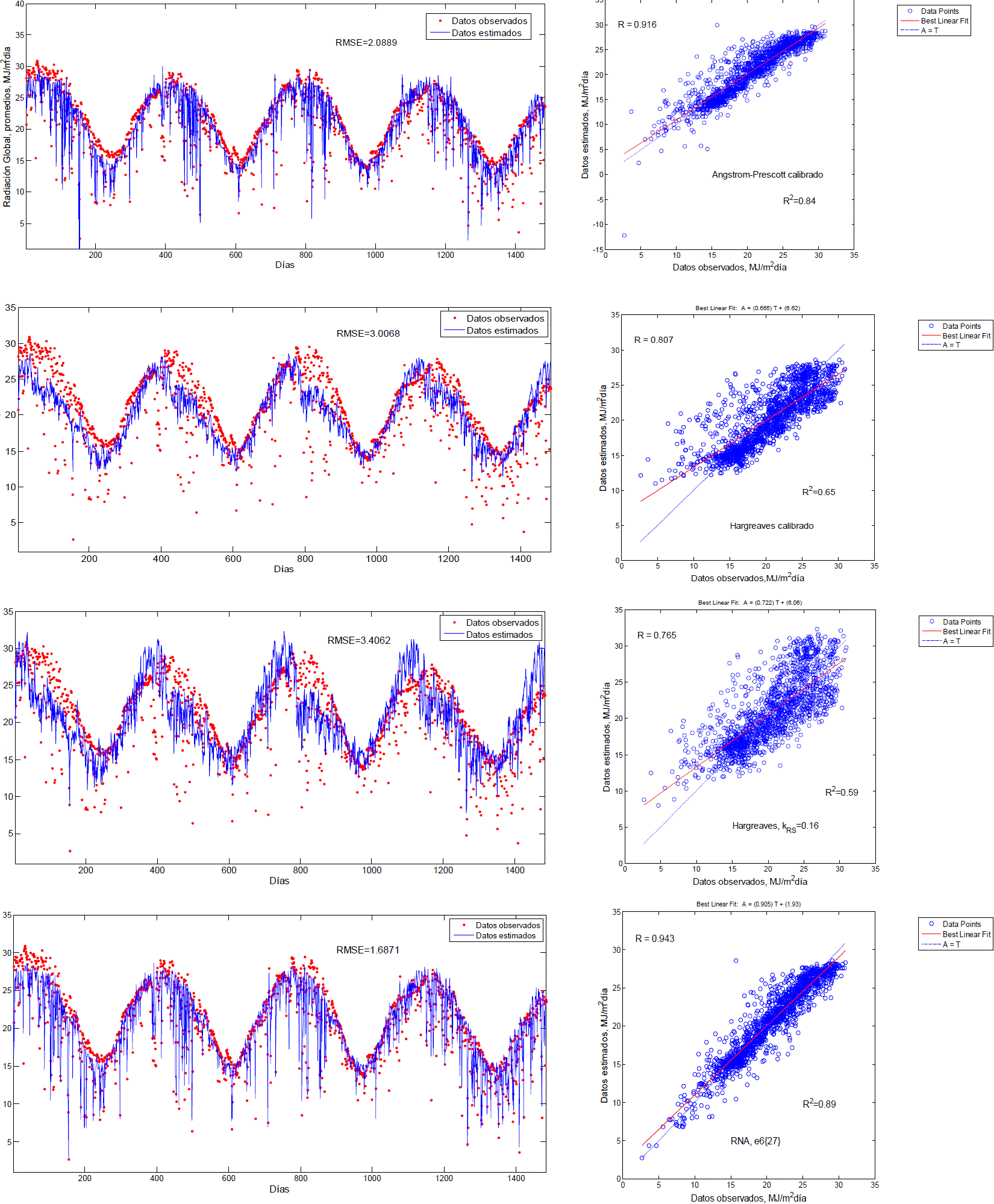
Figure 1 RMSE and R2 for estimates of Angström-Prescott models Hargreaves, Hargreaves calibrated with kRS= 0.16 and RNA e6{27} of the 1 484 average global radiation data.
In the Tables 2 and 3, it is observed that the best settings, mostly correspond to e5 scenarios and e6, which are those with more input variables, but also noted that a small number of input variables, such as maximum temperature and minimum temperature can make an acceptable prognosis of daily global radiation, with a variation of thousandths in the RMSE, but since there are weather stations that do not have an extensive range of instruments to measure all of climatological variables requiring e6 or e5 scenario, then a stage e2 is sufficient for prognosis. The Table 3 was formed with the same scenarios in Table 2, the first, second and third best fit observed in Table 3 were presented as follows: with three hidden layers, setting e15 with Tmax-Tmin, n/N, Ra, with 9x18x9 neurons in the hidden layers and a RMSE of 1.9847; the e2 entries with Tmin, Tmax, n, , with 9x24x9 in the hidden layers with a RMSE of 1.9918, and e15 with Tmax-Tmin, n/N, Ra with a hidden layer, and three neurons in it with a RMSE of 1.9939, although these do not match the best fits obtained in practice with 1 484 data. Jiang (2008) to estimate the diffuse solar radiation monthly average determined empirical models RMSE's of 0.783, 0.871 where the neural network model used, obtained a RMSE of 0.746, with the variables: index of daylight, percentage of hours brightness sun and output the average daily diffuse fraction.
Table 3 Standard error adjustment of the 229 observed data versus estimates RNA.
| # capas ocultas | Escenario 1er. mejor ajuste | RMSE | Escenario 2°. mejor ajuste | RMSE | Escenario 3er. mejor ajuste | RMSE |
| {3} | e2{Tmin, Tmax, n} | 2.3337 | e14{Tmin, Tmax, n, Ra} | 2.1491 | e15{Tmin, Tmax, n/N, Ra} | 1.9940 |
| {6} | e6{Tmin, Tmax, n/N, Ra} | 2.4499 | e5{Tmin, Tmax, n, Ra} | 2.2926 | e2{Tmin, Tmax, n} | 2.2473 |
| {9} | e6{{Tmin, Tmax, n/N, Ra} | 2.3480 | e5{Tmin, Tmax, n, Ra} | 2.2855 | e2{Tmin, Tmax, n} | 2.3655 |
| {12} | e6{{Tmin, Tmax, n/N, Ra} | 2.6696 | e5{Tmin, Tmax, n, Ra} | 2.4298 | e14{Tmin, Tmax, n, Ra} | 2.1303 |
| {15} | e14{Tmin, Tmax, n, Ra} | 2.0228 | e12{Tmin, Tmax, n} | 2.1793 | e5{Tmin, Tmax, n, Ra} | 2.6225 |
| {18} | e5{Tmin, Tmax, n, Ra} | 2.4279 | e2{Tmin, Tmax, n} | 2.2956 | e6{Tmin, Tmax, n/N, Ra} | 2.4736 |
| {21} | e6{Tmin, Tmax, n/N, Ra} | 2.5573 | e5{Tmin, Tmax, n, Ra} | 2.5344 | e14{Tmin, Tmax, n, Ra} | 2.1966 |
| {24} | e6{Tmin, Tmax, n/N, Ra} | 2.6016 | e5{Tmin, Tmax, n, Ra} | 2.5110 | e14{Tmin, Tmax, n, Ra} | 2.1684 |
| {27} | e6{Tmin, Tmax, n/N, Ra} | 2.5475 | e5{Tmin, Tmax, n, Ra} | 2.5316 | e15{Tmin, Tmax, n/N, Ra} | 2.1070 |
| {30} | e5{Tmin, Tmax, n, Ra} | 2.6182 | e6{Tmin, Tmax, n/N, Ra} | 2.6800 | e2{Tmin, Tmax, n} | 2.3271 |
| {3x3} | e5{Tmin, Tmax, n, Ra} | 2.1909 | e2{Tmin, Tmax, n} | 2.3395 | e6{Tmin, Tmax, n/N, Ra} | 2.2422 |
| {6x6} | e5{Tmin, Tmax, n, Ra} | 2.4623 | e2{Tmin, Tmax, n} | 2.2890 | e6{Tmin, Tmax, n/N, Ra} | 2.4429 |
| {9x9} | e6{Tmin, Tmax, n/N, Ra} | 2.4569 | e5{Tmin, Tmax, n, Ra} | 2.7467 | e14{Tmin, Tmax, n, Ra} | 2.1805 |
| {12x12} | e5{Tmin, Tmax, n, Ra} | 2.5214 | e6{Tmin, Tmax, n/N, Ra} | 2.3651 | e14{Tmin, Tmax, n, Ra} | 2.1963 |
| {15x15} | e6{Tmin, Tmax, n/N, Ra} | 2.6739 | e5{Tmin, Tmax, n, Ra} | 2.7528 | e2{Tmin, Tmax, n} | 2.4951 |
| {18x18} | e5{Tmin, Tmax, n, Ra} | 2.6202 | e2{Tmin, Tmax, n} | 2.3946 | e6{Tmin, Tmax, n/N, Ra} | 2.5563 |
| {21x21} | e14{Tmin, Tmax, n, Ra} | 2.1853 | e15{Tmin, Tmax, n/N, Ra} | 2.2015 | e2{Tmin, Tmax, n} | 2.1792 |
| {24x24} | e6{Tmin, Tmax, n/N, Ra} | 2.6534 | e2{Tmin, Tmax, n} | 2.3202 | e14{Tmin, Tmax, n, Ra} | 2.2036 |
| {27x27} | e5{Tmin, Tmax, n, Ra} | 2.6423 | e6{Tmin, Tmax, n/N, Ra} | 2.6350 | e14{Tmin, Tmax, n, Ra} | 2.5870 |
| {30x30} | e6{Tmin, Tmax, n/N, Ra} | 2.5884 | e5{Tmin, Tmax, n, Ra} | 2.8588 | e15{Tmin, Tmax, n/N, Ra} | 2.3436 |
| {3x3x3} | e14{Tmin, Tmax, n, Ra} | 2.1439 | e6{Tmin, Tmax, n/N, Ra} | 2.5014 | e2{Tmin, Tmax, n} | 2.3805 |
| {3x6x3} | e6{Tmin, Tmax, n/N, Ra} | 2.2795 | e2{Tmin, Tmax, n} | 2.4035 | e12{Tmin, Tmax, n} | 2.2951 |
| {6x9x6} | e6{Tmin, Tmax, n/N, Ra} | 2.3708 | e5{Tmin, Tmax, n, Ra} | 2.5424 | e14{Tmin, Tmax, n, Ra} | 2.1032 |
| {6x12x6} | e2{Tmin, Tmax, n} | 2.5072 | e14{Tmin, Tmax, n, Ra} | 2.2496 | e12{Tmin, Tmax, n} | 2.2698 |
| {6x15x6} | e5{Tmin, Tmax, n, Ra} | 2.4811 | e15{Tmin, Tmax, n/N, Ra} | 2.1214 | e6{Tmin, Tmax, n/N, Ra} | 2.3913 |
| {9x18x9} | e5{Tmin, Tmax, n, Ra} | 2.3122 | e15{Tmin, Tmax, n/N, Ra} | 1.9847 | e2{Tmin, Tmax, n} | 2.4131 |
| {9x21x9} | e5{Tmin, Tmax, n, Ra} | 2.4648 | e6{Tmin, Tmax, n/N, Ra} | 2.6346 | e15{Tmin, Tmax, n/N, Ra} | 2.0135 |
| {9x24x9} | e5{Tmin, Tmax, n, Ra} | 2.4281 | e6{Tmin, Tmax, n/N, Ra} | 2.4794 | e2{Tmin, Tmax, n} | 1.9918 |
| {9x27x9} | e5{Tmin, Tmax, n, Ra} | 2.6010 | e6{Tmin, Tmax, n/N, Ra} | 2.5653 | e14{Tmin, Tmax, n, Ra} | 2.0010 |
| {9x30x9} | e6{Tmin, Tmax, n/N, Ra} | 2.6286 | e2{Tmin, Tmax, n} | 2.3453 | e5{Tmin, Tmax, n, Ra} | 2.6287 |
Tmin= temperatura mínima; Tmax= temperatura máxima; n= horas brillo sol; N= fotoperiodo; Ra= radiación teórica extraterrestre; RMSE= raíz cuadrada del cuadrado medio del error.
In Figures 1 and 2 shows that the maximum and minimum temperature, with the figure for hours shine sun divided by photoperiod and extraterrestrial radiation (e6{27}) the best fit for training with 1484 vectors is reached data (R2 of 0.89 and RMSE of 1.6871), and the RNA and trained a new estimate of 229 data Rs (R2 of 0.88 and RMSE of 2.5475), which as shown in Table 3 is not for the best fit is performed results for global data 229, in this connection Senkal and Kuleli (2009) found correlation coefficient values for the training set and evaluation 0978 and 0971 respectively; and Fadare (2009) found values of the correlation coefficient and RMS (root mean square) for training 99.36% and 2.32 MJ m2 and for evaluation of 88.39% and 3.94 MJ/m2 respectively, indicating that all evaluation error values tend to grow.
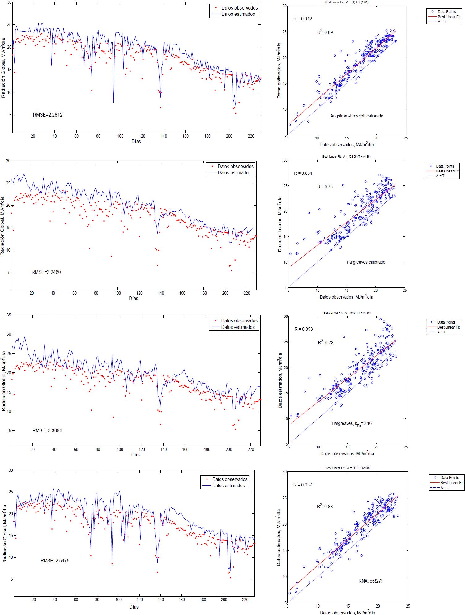
Figure 2 RMSE and R2 for estimates of Angström-Prescott models Hargreaves, Hargreaves calibrated with kRS= 0.16 and RNA e6{27} of the 229 average global radiation data.
Additionally in Figure 2 shows that both models calibrated Angström-Prescott models Hargreaves, Hargreaves calibrated and RNA including backpropagation overestimate the data observed daily global radiation. Tymvios et al. (2005) used three model variations Angström with different calibrated values for b and RNA performing training with different input variables including: month duration of hours brightness sun, maximum temperature and duration of hours brightness theoretical sun (photoperiod), their results they are similar to those found in this work; the artificial neural network model that used Tymvios et al. (2005) with the maximum temperature inputs, sun shine hours photoperiod measures and obtained an RMSE of 5.67%, followed closely by one of the models of Angström with RMSE of 5.81%. However Wan et al. (2008) found that the model of Angstrom calibrated in nine warm-seven areas with sunny weather in China, obtained a similar performance in the statistics RMSE and MBE fit with those found in this work, for 229 data, compared with the setting a neural network.
Conclusions
Invariably all workouts containing the variable sun shine hours (n) have a good fit.
The increase in hidden layers does not improve the setting value of RMSE, with one and two layers is sufficient to train an RNA for estimating daily global radiation.
The variables minimum temperature, maximum temperature and sun shine hours (n) are essential for a good prognosis of daily global radiation. Variable theoretical extraterrestrial radiation (Ra) is not relevant in the prognosis of daily global radiation.
For 1 484 average data, artificial neural network backpropagation in your scenario e6{27} presents the best estimate of daily global radiation (Rs), and is better than the empirical models, however for 229 forecast data, the Angström-Prescott calibrated model provides an estimate of Rs slightly better e6{27}.
Literatura citada
Alexandris, S.; Kerkides, P. and Liakatas, A. 2006. Daily reference evapotranspiration estimates by the “Copais” approach. Agric. Water Manage. 82:371-386. [ Links ]
Allen, G. R.; Pereira, S. L.; Raes, D. and Smith, M. 1998. Crop evapotranspiration Guidelines for computing crop water requirements. FAO Irrigation and drainage paper 56. Roma. 298 p. [ Links ]
Almorox, J.; Benito, M. and Hontoria, C. 2008. Estimation of global solar radiation in Venezuela. Interciencia 33:280-283. [ Links ]
Annandale, J. G.; Jovanovic, N. Z.; Benadé, N. and Allen, R. G. 2002. Software for missing data error analysis of Penman-Monteith reference evapotranspiration. Irrig. Sci. 21:57-67. [ Links ]
Bandyopadhyay, A.; Bhadra, A.; Raghuwanshi, N. S. and Singh, R. 2008. Estimation of monthly solar radiation from measured air temperatures extremes. Agricultural and forest meteorology, 148:1707-1718. [ Links ]
Benghanem, M; Mellit, A. and Alamri, S. N. 2009. ANN-based modeling and estimation of daily global solar radiation data: A case study. Energy Conversion Manage. 50:1644-1655. [ Links ]
Bristow, K. L. and Campbell, G. S. 1984. On the relationship between incoming solar radiation and daily maximum and minimum temperature. Agric. Forest Meteorol. 31:159-166. [ Links ]
Cervantes, O, R.; Arteaga, R, R.; Vázquez, P, M.A. y Ojeda, B. W. 2012. Radiación global diaria estimada con métodos convencionales y redes neuronales artificiales en el Distrito de Riego 075. Ingeniería Agrícola y Biosistemas. 4(2):55-60. [ Links ]
Demuth, H.; Beale, M. and Hagan, M. 2008. Neural network toolboxTM 6.User’s guide. 907 p. [ Links ]
Fadare, D. A. 2009. Modelling of solar energy potential in Nigeria using an artificial neural network model. Applied Energy. 86:1410-1422. [ Links ]
Hargreaves, G. H. and Samani, Z. A. 1982. Estimating potential evapotranspiration. J. Irrig. Drain. Eng., ASCE. 108(3):225-230. [ Links ]
Haykin, S. 2008. Neural networks: A comprehensive foundation. 2nd. Edition. Ed. Prentice Hall. United States of America. 842 p. [ Links ]
Hasni, A.; Sehli, A.; Draoui, B.; Bassou, A. and Amieur, B. 2012. Estimating global solar radiation using artificial neural network and climate data in the south-western region of Algeria. Energy Procedia. 18:531-537. [ Links ]
Jiang, Y. 2008. Prediction of monthly mean daily diffuse solar radiation using artificial neural networks and comparison with other empirical models. Energy Policy 36:3833-3837. [ Links ]
Linacre, E. 1992. Climate data and resources. A reference and guide. British Library Cataloguing in Publication Data. 170-172 pp. [ Links ]
Liu, X.; Mei, X.; Li, Y.; Zhang, Y.; Wang, Q.; Jensen, J. R. and Porter, J. R. 2009. Calibration of the Angström-Prescott coefficients (a,b) under different time scales and their impacts in estimating global solar radiation in the Yellow River basin. Agric. Forest Meteorol. 149:697-710. [ Links ]
Martínez, R, A.; Ortega, J. F.; de Juan, J. A.; Tarjuelo, J. M. y Moreno, M. A. 2012. Modelos de estimación de radiación solar global con limitación de datos y su distribución espacial en CastillaLa-Mancha. 108(4):426-449. [ Links ]
Meza, F. and Varas, E. 2000. Estimation of mean monthly solar global radiation as a function of temperature. Agricultural and forest meteorological. 100:231-241. [ Links ]
Muribu, J. 2008. Predicting total solar irradiation values using artificial neural networks. Renewable Energy. 33:2329-2332. [ Links ]
Rehman, S. and Mohandes, M. 2008. Artificial neural network estimation of global solar radiation using air temperature and relative humidity. Energy Policy. 36:571-576. [ Links ]
Senkal, O. and Kuleli, T. 2009. Estimation of solar radiation over Turkey using artificial neural network and satellite data. Applied Energy 86:1222-1228. [ Links ]
Tabari, H. 2009. Evaluation of reference crop evapotranspiration equations in various climates. Water Resour. Manag. 24:2311-2337. [ Links ]
Tymvios, F. S.; Jacovides, C. P.; Michaelides, S. C. and Skouteli, C. S. 2005. Comparative study of Angström’s and artificial neural networks’ methodologies in estimating global solar radiation. Solar Energy. 78:752-762. [ Links ]
Wan, K. K. W.; Hang, H. L.; Yang, L. and Lam, J. C. 2008. An analysis of thermal and solar zone radiation models using an AngstromPrescott equation and artificial neural networks. Energy. 33:1115-1127. [ Links ]
WMO. 1996. Guide to meteorological instruments and methods of observations, No. 8. Sixth edition. 157-198 pp. [ Links ]
Yadav, A. K. and Chandel, S. S. 2014. Solar radiation prediction using artificial neural network techniques: A review. Renewable and sustainable energy reviews. 33:772-781. [ Links ]
Received: April 2016; Accepted: June 2016
 Este es un artículo publicado en acceso abierto bajo una licencia Creative Commons
