


Serviços Personalizados
Journal
Artigo
 texto em
  Inglês (pdf)
 Artigo em XML
 Referências do artigo
 Enviar este artigo por email
Indicadores
-
 Citado por SciELO
 -
 Acessos
Links relacionados
-
 Similares em
SciELO
Similares em
SciELO
Compartilhar

 Permalink
Revista mexicana de ciencias agrícolas
versão impressa ISSN 2007-0934
Rev. Mex. Cienc. Agríc vol.7 no.4 Texcoco Mai./Jun. 2016
Articles
Analysis coefficients wind force and flow behavior on a greenhouse model
1 Ingeniería Agrícola y Uso Integral del Agua. Universidad Autónoma Chapingo. Carretera México-Texcoco, km 38.5, Chapingo, Estado de México, C. P. 56230, México. Tel: 5542956796.
2 Universidad Autónoma Chapingo, Departamento Ingeniería Mecánica Agrícola, km 38.5 carretera México-Texcoco 56230 Chapingo, Estado de México, México, C. P. 56230, (karlosvilla06@yahoo.com.mx; alelopez10@hotmail.com).
3 Universidad Autónoma Chapingo, Departamento de Irrigación, km 38.5 Carretera México-Texcoco, Chapingo, Estado de México, México, C. P. 56230, 01 595 95 2 1551.
4 INIFAP- Campo Experimental Valle de México, km 18.5 Carretera México-Lechería, C. P. 56230, A.P. 10, Estado de México. México. (rcervanteso@colpos.mx).
The greenhouses are usually constructed with plastic frames covered with metal and are also lightweight structures, which are sensitive to dynamic loads such as wind load. In this work the aerodynamic behavior of a model greenhouse with overhead vent is analyzed through the determination of local pressure wind tunnel using a scale model, considering different wind directions. Airflow on a greenhouse is a complex phenomenon, because this behavior airflow around the model was visualized by injection of smoke and the result was compared with a simulation performed on a software finite element (CFD) for a validation of the flow distribution; coefficients wind strength were determined and compared with values reported in some countries; corroborating the study. It is expected that the results will be useful for future research, and to ensure the mechanical safety of structures and be a benchmark for the industry of building greenhouses.
Keywords: CFD; downforce; greenhouse; simulation; smoke; wind tunnel
Los invernaderos usualmente se construyen con marcos de metal cubiertos con plástico y además son estructuras ligeras, por lo cual son sensibles a las cargas dinámicas tales como la carga de viento. En este trabajo se analiza el comportamiento aerodinámico de un modelo de invernadero con ventila cenital, a través de la determinación de las presiones locales en túnel de viento utilizando un modelo a escala, considerando distintas direcciones del viento. El flujo de aire sobre un invernadero es un fenómeno complejo, debido a esto se visualizó el comportamiento del flujo de aire alrededor del modelo por medio de inyección de humo y el resultado se comparó con una simulación realizada en un software de elemento finito (CFD) para obtener una validación de la distribución del flujo; los coeficientes de la fuerza del viento fueron determinados y comparados con los valores reportados en algunos países; corroborando el estudio. Se espera que los resultados presentados sean útiles para el desarrollo de futuras investigaciones, así como para garantizar la seguridad mecánica de las estructuras y ser un referente para la industria de la construcción de invernaderos.
Palabras clave: carga aerodinámica; CFD; humo; invernadero; túnel de viento; simulación
Introduction
Several authors have shown that greenhouses are built in the absence of construction project solely based on experience and local knowledge of construction companies (Briassoulis et al., 1997; Grafiadellis, 1999; Von Elsner et al., 2000; Kendirli, 2005; Yasemin-Emekli, 2010; Briassoulis et al., 2010). In the past, the development and design of greenhouses was mainly based on experience (Von Elsner et al., 2000). They all agree on the need to design conservatories according to regulations, or in line with the climatic conditions of the area, primarily serving the wind loads and snow. The very low weight of the greenhouses makes them especially vulnerable to high winds; events in those suffering damage ranging from avulsion to total collapse, as has been noted repeatedly.
For example, the wind generates pressure variations on the greenhouse cover and corresponding efforts in the framework and foundations, which can cause damage in case of extreme wind speeds. For this case the wind pressure is calculated as a function of the pressure coefficient corresponding housing segment into consideration and the dynamic pressure of wind. Wind loads appear as pressure and suction forces on the surface emissions. The wind dynamic pressure depends on the effective height of the greenhouse, which is defined as the distance between the ground level, the average height and the highest point of the roof (Von Elsner, 2000; ENV, 2002; Subramani and Sugathan, 2012).
One of the most destructive forces around a greenhouse is the wind; wind loads can be calculated by the free flow pressure multiplied by the coefficient of the wind. Coefficients depend on the wind direction, so the greenhouse, size, and presence or absence of vents and windbreaks. Generally, they can be determined in experiments in wind tunnel. The reported values show differences in some countries due to the experimental conditions. In particular, greenhouses covered with plastics are very light structures and often experience damage from windstorms. The wind pressure coefficient is used in the design of the greenhouses to improve the structures thereof. The appropriate estimate of the distribution coefficient wind pressure depends on the shape of the structure, measurements at full scale, dynamic analysis computational fluid and testing wind tunnel for different types of greenhouses covered with plastics (Hoxey et al., 1984; ASAE Standards, 1987; Mathews et al., 1987; Mistriotis et al., 2002; Robertson et al., 2002; Brugger et al., 2005; Allori et al., 2011). Moriyama et al. (2010) conducted a wind tunnel test to obtain the distribution coefficient of wind pressure on a greenhouse.
It should be noted that several standards adopted different approaches for calculating wind loads. As a result the design loads may differ significantly. Depending on the geometric shape of the aerodynamic coefficients construction must consider for the pressure surface of each sector structure.
The purpose of this study was to determine the coefficients of the wind on a type of greenhouse with typical overhead vents in the central area of Mexico, by building a scale model, instrumented with pressure taps in a tunnel test wind; the results are considered very useful for optimizing the structures of the greenhouses, and to ensure the mechanical safety also were compared with values reported by other studies, the results of downforce are also displayed per unit area using the results of the coefficients of average pressure and pattern display airflow around the structure. The study by the finite element method, was intended to compare the results of the coefficients and distribution of wind load, obtained in the wind tunnel test.
Materials and methods
The tests were conducted in the framework of the methodology presented by Barlow et al. (1999) in the wind tunnel PA-2ZU suction with test section of 1.2 x 1.2 x 2.4 m in high school of Mechanical and Electrical Engineering, Unit Ticoman. The wind tunnel developed a wind speed of 95.34 km h-1. The scale model of a common greenhouse built in Mexico was 1:100 with 22 pressure taps as shown in Figure 1. The corresponding full scale model has dimensions of 7.5 m wide, 6.22 m high crest and 42 m in length; the stagnation effect on the pressure distributions was considered insignificant (Jensen et al., 1995).
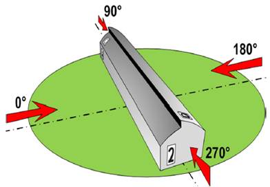
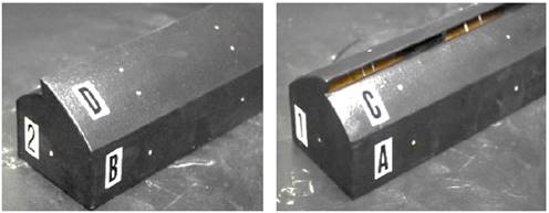
The model was made of wood, for 4 measurements were performed angular positions with respect to the wind direction to 0, 90, 180 and 270° (Figure 1); model surfaces are defined in Figure 2.
The environmental conditions during the test averages were as follows (Table 1).
Table 1 Environmental conditions during the test.
| Parámetro | Valor promedio |
| Temperatura ambiente | 19.6 °C |
| Presión atmosférica | 587.5 mmHg |
| Humedad relativa | 79% |
| Densidad del aire | 0.923 kg m-3 |
For measurement of local pressures pressure taps connected by capillaries PVC, multicolumn manometers were used. The profile of the average wind speed at a height of 1 m in the center of the turntable wind tunnel was measured by an anemometer (IFA300 model, TSI, Inc.). The influence of Reynolds number on the wind pressure was assumed negligible (Building Center of Japan, 1994). The test was carried out without boundary layer terrestrial simulation. The coefficient of wind pressure can be defined as follows (Equation 1):
Where: Cp= coefficient of wind pressure; p= the pressure acting on the model (N m-2); Ps= static pressure on the wind tunnel (N m-2); qh= free flow pressure (N m-2); ρ= air density (kg m-3); UH= wind speed at reference height (m s-1).
The static pressure was measured by a pitot tube located at a point 3.5 m below the center of the turntable. The estimated coefficients in the wind direction to 0, 90, 180 and 270° (Figure 3), were compared with the values provided by ASAE (1976); JGHA (1981); ANSI (1982) and Nelson (1988).
Pattern display airflow
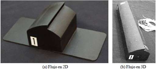
The airflow around a structure is complex and difficult to understand the flow field only from the distribution of the pressure coefficients. For a better appreciation of the relationship between the air flow and the geometry of the greenhouse, visualization was performed by injection of smoke in two and three dimensions:
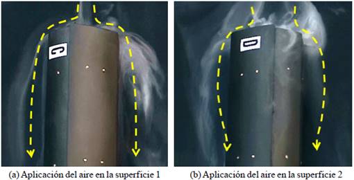
1) The 2D flow visualization. This method is not considered the influence of the model ends, the faces 1 and 2 coincide with the walls of the section of the wind tunnel (Figure 2).
2) The 3D flow visualization. As in the coefficients of pressure surfaces for 3D flow model they are defined as shown in Figure 3. To display one video stream commercial Sony SLT A77 V Co., Ltd. was used, and smoke generator and injector high speed.
The load per unit area is obtained with Equation 2:
Where: p= downforce per unit area (N m-2); and q= the dynamic pressure of free flow (N m-2).
To validate the flow behavior around the geometry simulation was performed using the software Ansys Version 12, under the same conditions both flow rate and environmental, as for testing in the wind tunnel.
Results and discussion
Comparison of the coefficients of the wind
The geometry for items a), b), c) and d) of Figure 3 are arch type, present likeness; These studies were conducted for different latitudes, even so, there is variation in the results, these are attributed to the dissimilar experimental conditions such as: testing in the wind tunnel, the boundary layer, the Reynolds number, roughness model, the location of the pressure taps and measurement methods (Lee and Lee, 1996). We must emphasize the negative coefficient of subsection e) Figure 3, which is not presented in the studies cited above, this coefficient is of the vortices that are generated in the leeward area which is corroborated by numerical simulation.
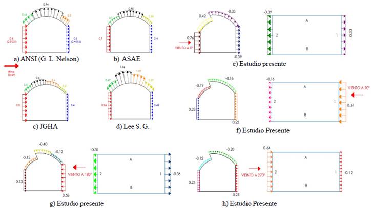
In the Figure 4 shows the distribution of the coefficients of the wind compared to studies by different authors. The values of the coefficients on the wall to windward showed discrepancies. Lee and Lee (1996), Lee (2005) and Nelson (1998) presented results of 0.5 to 0.6, and 0.5 to 0.8 respectively. The results as those reported by Nelson (1988), ASAE (1976) and JGHA (1981), showed average values of 0.7 to 0.8, unlike the results reported by Lee (1996), whose average value was 0.55 .
Because the distribution of the wind pressure on the walls vary in thickness windward boundary layer and the height of the wall, considered coincident proposed by Nelson (1998) and Lee (1996) values. In this range of values are the average value of the windward wall for the typical greenhouse with overhead vents built in Mexico.
The coefficients obtained in lower arch windward in a quarter of the width of the roof, were similar to those reported by Lee (1996), JGHA (1981) and ANSI (1982), and they were very different from those presented by ASAE (1976). In the middle region of significant discrepancies they were found, which are mainly attributed to differences in the experimental conditions for testing wind tunnel, such as the Reynolds number, the type of terrain, surface model greenhouse, location taking pressure, and measurement methods. To top leeward bow in a quarter of the width of the roof, the results were similar to those reported by JHGA (1981), and showed inconsistency with those presented by Lee (1996), ANSI (1982) and ASAE (1976). The coefficients obtained on the leeward wall were similar to the results reported by these authors.
For baseline studies only estimate the wind direction was held at 0° for which there are no comparative results with the following angular positions described above. According to Ha et al., (2014), in a test wind tunnel for a greenhouse with three porches with wind direction at 0 and 90°, the maximum value reached Cp was 0.48, with very high suctions up -1.39 in the orientation 0°.
The following observations were considered important:
The pressure coefficients obtained can be used under any speed value, the model geometry shows no dependence on the Reynolds number. In the time period of measurements, the results were found to exhibit stability over pressure coefficients. It is remarkable the case of flow affecting 180°, a peculiar case is presented where the surface A leeward, presents positive values of Cp, lower than those of the B surface windward due to the difference in heights C and D surfaces, and the arc shape (Figure 3g).
Three critical cases were analyzed: Positive maximum load was presented at 0° on the surface A, due to the direct position on the windward side of the overhead vent, which generated a tendency to stagnation, producing high values of Cp (Figure 3e). The negative maximum load was also presented at 0° on the side surface 2 and B leeward surface (Figure 3e). Finally the negative maximum load was
also presented at the 180° of incidence of the wind, specifically on top of the surface D, caused by the vigorous evolution of flow exists in that area (Figure 3g). The positive value of Cp on the roof windward and high suction on the roof leeward, caused a large drag on the frames which can cause buckling or collapse under a low wind speed, as in an isolated frame (Figure 3e). Therefore, the arc near the wall should be reinforced, or leeward column design.
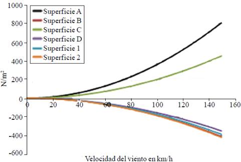
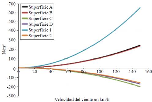
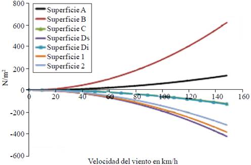
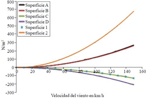
The load per unit area is shown in Figures 5-8, for each zone of incidence of the wind, the importance of the results of these graphs is that they can be used directly by designers geometries in greenhouses central Mexico, it is observed that the maximum load occurs on the surface a (Figure 5), it follows that at a given wind speed corresponds to a value of pressure head design, likewise for each of the figures different incidents of wind flow.
Airflow display 2D smoke obtained by injection
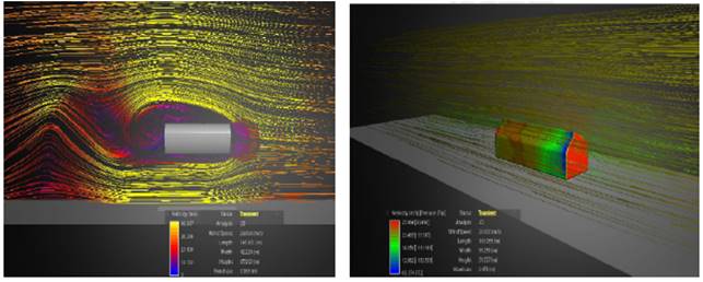
In Figure 9a vortices detached from the top of the model, generated in an area of depression leeward observed. In Figura 9b vortices generated by the shedding flow on top of the vent shown. Note that the number 1 in reflection position is that the model turned 180° in the tunnel and photographic equipment captured in the model inverted. Finally he was given a digital treatment of the image to match the flow direction to the first case analyzed (direction from right to left).
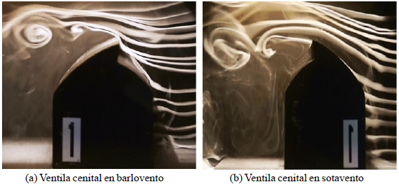
Figure 9 Vortices generated at the top by the evolution model of the flow. Airflow display 3D obtained by injection smoke.
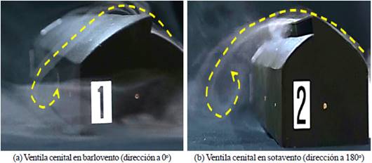
In the Figure 10a presents the three-dimensional air flow at 0°, and greater adherence of the lines of current compared to the case of two-dimensional flow is observed. Figure 10b shows the three-dimensional air flow 180°, and a vortex larger is observed to the case of direction 0°. Figure 11 presents in both cases a detached flow at the corners, generating vortices adjacent to these, having very low influence asymmetric condition of the awning.
Air flow simulation obtained 2D finite element
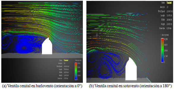
The flow behavior oriented at 0°, denotes the generation of a series of vortices due to the geometry having the overhead vent, resulting in a negative pressure acting on the leeward shaped drag (Figure 12). Can be seen just vortices generation area depression, causing turbulence wake quite long compared to the width of the cross section. A 180° vortices are also appreciated, the difference is its development, its diameter is increasing rapidly and are directed towards the ground with a steep slope, the last vortex opens and this causes a region of reverse flow impact to the side model, which is consistent with the positive values of Cp (Figures 3a and 12).
Air flow simulation obtained 3D finite element
The distribution of free flow and the pressure exerted on the model with an orientation of 0°, was distributed in the windward area, being the most critical value in the center, showing a downward trend towards the banks. Leeward negative pressure zone due to vortices emerging from the top of the same geometry (Figure 13a) can be seen. Also here the vortices are seen, but its trajectory is steeper toward the ground, generating this an area downwind with a value of positive pressure coefficient.
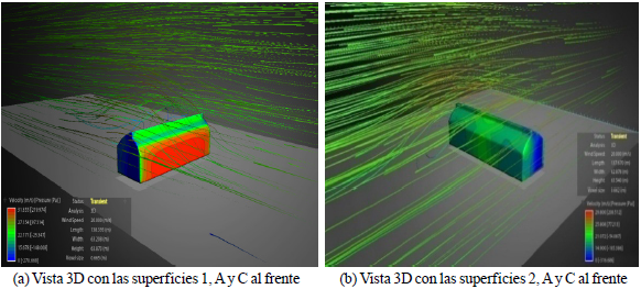
Figure 13 Finite element simulation of the air currents in regard to windward aerial vents (flow orientation at 0°).
When the orientation of the wind flow direction 180°, an increase in the value of the negative pressure affects leeward, because the vortex generated is larger compared with that obtained in the direction of 0° it is observed (Figure 13b). For areas defined as 1 and 2 predominates detachment flow just around the corner, with a tendency to adhere downstream, tending qualitatively to be a similarity between the experiment in wind tunnel and simulation in CFD (Figures 14a and 14b). As Ha et al. (2014), the values obtained from the distribution of Cp simulation CFD and visualization airflow, were qualitatively similar but for comparison is necessary to improve the CFD model. The study display both smoke injection as computed by numerical simulation, coincided with the data distribution coefficients reported pressure.
Conclusions
In this study, the distribution coefficients air pressure along surfaces greenhouse model was determined, these were calculated by a test in a wind tunnel which simulates the flow; generally calculated values are within an acceptable range. The flow distribution to the numerical simulation and the average values of the coefficients compared with other studies; a critical peak load positive case was brought to 0° incidence surface wind A due to direct windward position in the overhead vent.
And the downforce was determined per unit area which will be useful for builders evaluate and suggest a new design plan taking the structural stability into account.
Literatura citada
Allori, D.; Bartoli, G. and Miguel, A. F. 2011. Fluid flow through macro-porous materials: friction coefficient and wind tunnel similitude criteria. Int. J. Fluid Mech. Res. 39(2):136-148. [ Links ]
Allori, D.; Bartoli, G. and Mannini, C. 2013. Wind tunnel tests on macro-porous structural elements: a scaling procedure. J. Wind Eng. Ind. Aerodyn. 123:291-299. [ Links ]
American National Standards Institute. 1982. Minimum design loads for buildings and other structures. ANSI 58.1. New York, N.Y, United States. 100 p. [ Links ]
American Society of Agricultural Engineers. 1976. Designing building to resist snow and wind loads. ASAE. United States. 373-377 pp. [ Links ]
Barlow, J. B.; Rae, W. H. and Pope, A. 1999. Low-speed wind tunnel testing. 3rd ed. Wiley. New York, USA. 713 p. [ Links ]
Belloli, M.; Rosa, L. and Zasso, A. 2014. Wind loads and vortex shedding analysis on the effects of the porosity on a high slender tower. J. Wind Eng. Ind. Aerodyn. 126:75-86. [ Links ]
Briassoulis, D.; Waaijenber, J.; Gratraud, J. and Von Eslner, B. 1997. Mechanical properties of covering material for greenhouses: part 1. General overview. J. Agric. Eng. Res. 67(3):81-96. [ Links ]
Briassoulis, D.; Mistriotis, A. and Giannoulis, A. 2010. Wind forces on porous elevated panels. J. Wind Eng. Ind. Aerodyn. 98(12):919- 928. [ Links ]
Brugger, M. J.; Montero, E.; Baeza, J. and Pérez, P. 2005. Computational fluid dynamic modelling to improve the design of the spanish parral style greenhouse. Acta Horticulturae 691:425-431. [ Links ]
Building center of Japan. 1994. Guidebook of wind tunnel test for building. Tokio, Japan. [ Links ]
ENV 1991-1. 2002. Eurocode 1: basis of design and actions on structures: basis of design. European Committee for standardization CEN. Brussels, Belgium. 61-70 pp. [ Links ]
Fluent. 2013. Fluent documentation. Fluent Inc. Lebanon. N. H. USA. 1864 p. [ Links ]
Grafiadellis, M. 1999. The greenhouse structures in Mediterranean regions-problems and trends. Cahiers Options Mediterraneennes. 31:17-27. [ Links ]
Ha, T.; Lee, I. B.; Hwang, H. and Ha, J. 2014. Wind pressure coefficients determination for greenhouse built on a reclaimed land. Acta Hortic, 1037:1001-1008. [ Links ]
Hoxey, R. P. and Richardson, G. M. 1984. Measurements of wind load son pull-scale film plastic. Ciad. greenhouse. J. Wind Eng. Ind- Aerodyn. 16(1):57-83. [ Links ]
Japan Greenhouse Horticulture Association, 1981. Greenhouse structural requirement. JGHA. Japón. 12-17 pp. [ Links ]
Jensen, M. and Grank, N. 1995. Model-scale tests in turbulent wind: part II. Danish technical press. Copenhagen, Denmark. 97 p. [ Links ]
Kendirli, B. 2005. Structural analysis of greenhouses: a case study in Turkey. Build Environ. 75(1):1-16. [ Links ]
Lee, S. G. and Lee, H. W. 1996. An analysis of wind force coefficients for structural design of greenhouse. Acta Hortic. 440:280- 285. [ Links ]
Lee, I.; Lee, S.; Kim, G.; Sung, J.; Sung, S. and Yoon, Y. 2005. PIV verification of green- house ventilation air flows to evaluate CFD accuracy. Transactions of the ASAE. 48(5):2277-2288. [ Links ]
Mathews, E. H. and Meyer, J. P. 1987. Numerical modeling of wind loading on a film clad greenhouse. Bldg. Environ. 22(2):129- 134. [ Links ]
Mistriotis, A. and Briassoulis, D. 2002. Numerical estimation of the internal and external aerodynamic coefficients of a tunnel greenhouse structure with opening. Comp. Electric. Agric. 34(1):191-205. [ Links ]
Moniyama, H.; Sase, S; Uematsu, Y. and Yamaguchi, T. 2010. Wind tunnel study of the interaction of twoor three side by side pipe - framed greenhouses on wind pressure coefficients. Transactions of the ASABE. 53(2):585-592. [ Links ]
Nelson, G. L.; Manbeck, H. B. and Meador, N. F. 1988. Light agricultural and industrial structures. Van Nostrand Reinhold Co. Netherlands. 147-161 pp. [ Links ]
Robertson, A. P.; Roux, J.; Gratraud, G.; Sxarascia, S.; Castellano, M.; De Virel, D. and Palier, P. 2002. Wind pressures on permeably and impermeably-clad structures. J. Wind Eng. Ind. Aerodyn. 90(4-5):461-474. [ Links ]
Subramani, T. and Sugathan, A. 2012. Finite element analysis of thin walled-shell structures by ANSYS and LS-DYNA. Int. J. Moder. Eng. Res. (IJMER). 2(4):1576-1587. [ Links ]
Von Elsner, B.; Briassoulis, D.; Waaijenberg, D.; Mistriotis, A.; Von Zabelititz, C.; Gratraud, J.; Russo G. and Suay-Cortes, R. 2000. Review of structural and functional characteristics of greenhouses in European Union countries, part I: desing requirements. J Agric. Eng. Res. 75(1):1-16. [ Links ]
Received: January 2016; Accepted: May 2016
 Este es un artículo publicado en acceso abierto bajo una licencia Creative Commons
