Background

^{Busbice (1970)} showed that the genotypic value is:

G= A + (1 - F)B

Where: F= coefficient of inbreeding; A= additive component; and B= heterozygous component. When B= 1 there is additivity only in the genotype. Thus the overall additivity is manifested, for example, in the lines obtained over many self-fecundations. In practice the selection of the additive increases the response (R) to the selection, since as stated, after each cycle plants are increasingly related.

Additivity (A) in the selection cycle t is equal to the sum of the additive and the response (R) to the selection in the immediately preceding cycle:

On the right side of Equation [1] to the term (1 - F) B is called heterozygosity and varies from zero to B. Heterozygosity was defined by Falconer (1964) as "the frequency of heterozygous at any time in relation frequency in the population base”. Therefore, as the selection progresses inbreeding increases while heterozygosity is reduced.

In ^{Hallauer et al. (2010)}, the reduction in yield in the BSSS population varied from 0-100% of homozygosity, which caused the reduction in the yield of 70 quintals per hectare equal to 20/70 = 28%, which meant a heterozygosity of 72%. In this manuscript were taken as a basis the respective approaches 30 and 70%.

The coefficient of inbreeding (^{Márquez- Sánchez, 2008}) in cycle t selection for families n and m plants per family was calculated as:

Equation [2] is based on the constitution of a maize variety, as a population of sib families.

For the calculation of the response to the selection, the numbers n and m of Equation [2] must be adjusted for the actual number of variance according to ^{Crossa and Venkovsky (1997)}.

Without the influence of genotypic mean inbreeding in the selection t cycle is YtS, calculated as the average of the previous cycle Yt-1S plus the response to the selection in the same cycle (R_t-1), i.e.:

Response to selection

^{Márquez- Sánchez (2008)} adaptation of the response equation for mass selection is a gene locus (^{Empig et al., 1971}):

RSM=4iu2p(1-p)3/σP

Where= i is the selection intensity; u= the semidifference between the genotypic values of homozygous dominant and the recessive homozygote; p= is the gene frequency and σ is the standard deviation P phenotype. Considering each a k loci, everyone with a frequency of 0.5 (^{Goodrich et al., 1975}) determining the character, then ku= U. Therefore, in cycle t of selection the answer is:

The mean and phenotypic variance at the plant level were calculated with data from the doctoral thesis of ^{Márquez-Sánchez (1969)}, with mean Y= 150 g, and σ 2 P= 228675.24 g (σ P= 478.2 g). The response to selection depends on the selection pressure in this study is: s= 5%, which corresponds to a selection intensity i= 2.08; also depends on the percentage value of the response in the cycle 0, approximately equal to 2, as already mentioned. With this information the value of U², which also assumed complete dominance obtained as ^{Gardner and Lonnquist (1959)} found that there were approximately complete dominance, in a population derived from several generations of genetic recombination of the original cross. To calculate U², the percentage response selection cycle 0 was used, that is:

RSM%=4iU2p01-p03/σP/Y=0.02=(4×2.08×0.0625)U2/478.2/150=0.02=(0.000007249)U2=0.02

Where: U²= 2759.0012; knowing i, U², σ_P and Y= the absolute response in the cycle depends only on pt, and it is:

Inbreeding influence

Inbreeding is calculated using Equation [2], and as mentioned, the values of n and m must be set by the effective number of variance by:

Ne(v)=nm[4s/(1+2s)]

As mass selection generally used n= 200 and m= 20, nm= 4 000, is obtained:

Ne(v)=727.27

Adjusted numbers are n*= 85 280 and m*= 8528 according to ^{Márquez-Sánchez (2010)}, so the working equation of Equation [2] is:

Finally, affected by genetic inbreeding half cycle t is calculated from the equation G= A + (1 - F) B, as:

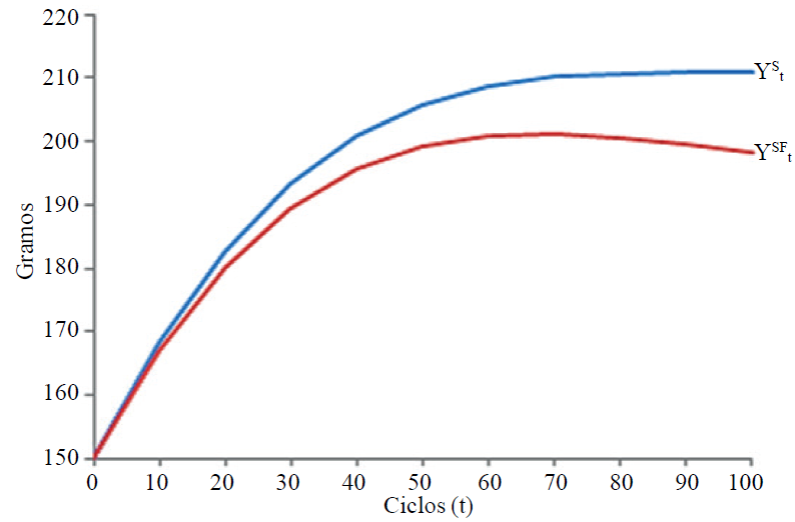
The Table 1 shows yields at 100 cycles of selection in each tenth cycle, are also shown: the gene frequency (pt), the response to selection (R_t) calculated with Equation [5], additivity (A_t) calculated with Equation [1], and S_t calculated with Equation [3], F _t calculated with Equation [6] and YtSF calculated with Equation [7].

Table 1 Parameters used for calculating the genotypic means without the effect of inbreeding (YtS) and with the effect of inbreeding (YtSF), in the t cycle of selection during 100 cycles in each tenth cycle. 

It is noted that, the value of R_t is reduced to zero in the cycle 100, YtS, At and Ft increase with the selection cycles. The Figure 1 shows how YtSF starts to decrease in the cycle 67. The effect of inbreeding, reduce yield, is clearly shown as YtSF except in the cycle 0, is always lower tan YtS while 11.76% is the total effect of inbreeding in the cycle 100.

Figure 1 Yields of YtS and YtSF in 100 cycles of mass selection. 

It is expected that, the effect of inbreeding also manifest in other characters that were not included in this research.

Conclusions

The influence of inbreeding is clearly stated as over selection cycles always existed a positive difference between the income of the means unaffected by inbreeding and means affected by it. This influence on the selection cycle 100 was 11.76%.