Introduction

The estimate of runoff depth is an intermediate calculation process so that together with methodologies such as the hydro-gram unit, can be estimated the increasing or flood, which has several practical applications, among which are: the determination of the flood to be use in the design flood drain and the forecasting of floods in real time (^{McCuen, 2004}; ^{Juárez et al., 2009}; ^{Miranda et al., 2009}). Moreover, the HMS software (^{USACE, 2000}; ^{USACE, 2010}), which is quite popular, employs such method for estimating of floods per event. To this end, with HEC-HMS, the basin is delimited, it is divided into sub-basins and for each requires the Nc.

The reason why the HEC-HMS do not generalizes, requiring only one NC for the entire basin is because by applying a NC by sub-basin ensures that calculations are the most accurate according to the conditions that dictate the hydrological response of what is called hydrological response unit, UHR (^{Neitsch et al., 2011}). Other popular software, which is the SWAT only calculates the runoff under two methods: runoff curve and Green-Ampt (^{Neitsch et al., 2011}); with this software, the basin is also delimited, it is divided into sub-basins and each sub basin is divided into UHR, requiring a Nc for each.

The number of runoff curve method for estimating then runoff depth is based on tabulated values of Nc, developed by the late Soil Conservation Service (SCS), US for basins on the territory of that country; where the number of curve chosen will depend, in practical terms, on the soil texture (hydrologic soil group), land-use, density of vegetation cover (hydrological conditions) and the possible existence of conservation practices of soils. The Nc thus determined, must be corrected by the average slope of the basin and the rain of the previous five days (antecedent moisture condition, CHA). However, when choosing the number of runoff curve in some land uses, tables are very general; for example, there is a category called "forest or jungle" and often fall into that category, leading to a generality that can cause errors.

For that reason, it is important to identify Nc for very specific hydrological response units categories, ie specific types of soil and vegetation cover, instead of doing it for the entire basin, which could only be useful for expeditious and general calculations for basin. The allocation of a specific Nc for the UHR, which is common in a watershed, would add one more category to the boards of SCS according to the conditions of the basin of interest.

The use of the concept of number of runoff curve Nc, defined by the Soil Conservation Service (SCS) (^{Mockus, 1949}; ^{Campos, 2002}; ^{Neitsch et al., 2011}; ^{Natural Resources Conservation Service, 2013}) is an alternative for the calculation of runoff, and used by several authors in many countries. The Nc given for estimating drained sheet can be found in tables reported by ^{McCuen (2004)} and ^{Campos (2002)}. The concept of Nc estimated based on rainfall data and soil characteristics in basins where no capacity data is abailable (^{Dal-Ré, 2003} and ^{Arellano, 2012)}. However, it does not give the expected results because the values defined by the SCS are not suitable for tropical areas (^{Muzik, 1993}). Although it has the advantages of being predictive, stable and require a single parameter, its disadvantages are: 1) the runoff values are very sensitive to a change in Nc; 2) lack detailed information on their variation for different precedent moisture conditions CHA; 3) lack of precision of the method for different coverages; 4) lack of knowledge of how space affects the scale of application Nc and; 5) development was done in specific conditions, which is not regionalized based on geology and climate, so it should be reviewed for each region (^{Ponce and Hawkins, 1996}). According to Mockus, one of the authors of the method, interviewed by ^{Ponce (1996)}, this work was generated with the Soil Conservation Service of the United States that began in 1928 in several parts of the territory of the United States and covered a period of 10 and 20 years for various sites. Mockus said it was not expected that the method was a predictor of infiltration but the total runoff volume, and this estimate is an average trend and not an exact value of an individual event.

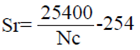
The number of runoff curve (Nc, dimensionless) is defined as a function of the potential retention (Sr, in mm) of rain on the part of the basin (^{McCuen, 2004}):

)1

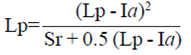
The Sr depends on soil conditions, vegetation cover and crop management and is calculated using Equation 2 (^{Neitsch et al., 2011}) or, Equation 3, developed by ^{Hawkins (1993)}, for the determination or field calibration of Nc.

)2

)3

For any data, Lp, Le, in the range of (0 <Le <Lp), where Lp is the precipitated sheet in mm, and Le is the runoff depth in mm.

In the Nc tables, the hydrological condition refers to the density of vegetation cover, which is a very common use in the categories of forest, jungle and pasture; and regular hydrologic condition refers to densities between 50 and 75% (^{McCuen, 2004}). The hydrologic soil group (^{McCuen, 2004}) can be A, B, C or D and the group can be defined according to any of the following criteria: a) texture; b) infiltration rate; c) if it is in the United States according to the county. In Mexico it is quite common to use it for texture. Group A are sandy soils, group B are loam, Group C are clay soils, and the group D are highly plastic clay soils.

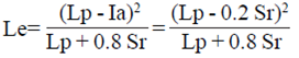
The direct surface runoff is estimated as a non-linear function of the precipitation Lp and from the so called initial abstractions (Ia) with equation 4, depending on the moisture content of the soil, land-use and soil type (^{Arellano, 2012}). Ia is calculated using Equation 5 with λ = 0.2 and, the Ve, is obtained from equation 6, wherein Ac is the area of the basin.

)4

For Lp> Ia, otherwise Le= 0.

)5

)6

In order to extend the applicability of the method to other conditions, ^{Mishra et al. (2005)} reviewed the methodology of Nc on the SCS using data coming from basins with areas of between 0.3 and 30.351 ha and rainfall data of 179 events registered from 1 to 50 years; discretized the precipitation (Lp, in mm) into five classes according to their size: Class A events with Lp <= 12.7, Class B for Pr between 12.7 and 25.4, C Class for Lp between 25.4 and 38.1, Class D for Lp between 38.1 and 50.8, and Class E for Lp> 50.8; and proposed Equation 7 to calculate Le, and for that of λ of equation 5 raised use the median rain event in the basin; finding that for the events with more than 38.1 mm Lp, Equation 4 works well, but in general for all events works best the equation 7 (^{Mishra et al., 2005}):

)7

Meanwhile, ^{Paz-Pellat (2009)}, made an analysis of the equations of SCS associated with Nc, concluding that no hydrological support as it is a result of the null hypothesis of equal two straight lines (Le= Lp and Le= Lp - Sr), which is possible only when Sr tends to zero and Lp to infinity.

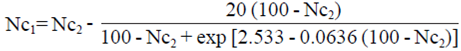
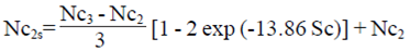
The Nc varies with soil moisture content, from their minimum values when the soil is permanent wilting point (PMP) to about 100 when soils are saturated (^{Neitsch et al., 2011}), so we should evaluate the antecedent moisture condition (CHA) in which events occur. According to ^{McCuen (2004)} and ^{Aparicio (2012)} the SCS defines three situations CHA, associating them to the hasty sheet (Lp), 5 days before the event date analyzed: I dry, corresponding to PMP, equivalent to one Lp <25 mm; II Average humidity, equal to Lp between 25 and 50 mm and; III wet, corresponding to the soil field capacity (CC) and equivalent to more than 50 mm of Lp. The Nc is calculated using Equation 8 for the moisture condition I and is called Nc₁, equation 9 for the moisture condition III and called Nc₃ while Nc₂, when it refers to the condition II and corresponds to the obtained SCS tables. The equations are (^{Neitsch et al., 2011}):

)8

)9

When the slope is higher than 5%, the Nc₂ obtained from the tables must be adjusted using Equation 10 (^{Neitsch et al., 2011}):

)10

Where: Nc_2s is the number of curve for the moisture condition II, adjusted for slope and Sc is the average slope of the land in the watershed, dimensionless. In order to calculate the adjusted Nc by slpoes for the antecedent moisture conditions I and III, the equations 8 and 9 are used, but replacing Nc_2s instead of Nc₂.

In the upper basin of the river Huehuetán, Chiapas, neighbor of the Basin Huixtla, ^{Arellano (2012)} calibrated the Nc for three micro-watersheds implemented, obtaining Nc= 63 for a dense forest with high evapotranspiration for soil hydrological conditions between C and D; 46 for acahual, corresponding to a sparse forest with low evapotranspiration for a hydrological soil condition A; and 77 for mango-grass cover, which corresponds to a sparse natural forest with low evapotranspiration and soil condition between B (with Nc = 73) and C (Nc = 82) according to Table 2. Also for Chiapas coast, ^{Campos (2010)} estimated the Nc from data in 24 h maximum rainfall for the basin of the river Despoblado, with thick forest coverage with high breathability and hydrological group between C and D (Nc= 64) and Coatán (Nc= 58) with very thick forest condition with high breathability and hydrological group between C and D of the SCS.

Table 1 Characteristics of the micro-watersheds Rosita, Hannover and Berriozabal. 

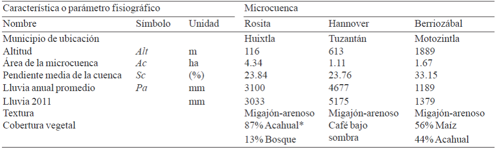
*El acahual o huatal, se refiere a la vegetación secundaria de la selva baja caducifolia que rebrota cuando el terreno está en descanso (barbecho) en el sistema de roza-tumba y quema (Waibel, citado por ^{Arellano, 2012}).

Table 2 Statistical information on the events used to calculate the runoff curve. 

^{Ares et al. (2012)} calibrated the Nc in an agricultural watershed in the province of Buenos Aires, Argentina, with an area of 116 km², average slope of 2.8%, elevation between 340 and 188 m and soils with infiltration rates between 60 and 24 mm/h; analyzed 108 events occurred between 2001 and 2007 and concluded that it is necessary to determine the Nc with local data. ^{Guichard et al., 2014}, calibrated the numbers of runoff curve in micro-watersheds of the Coast of Chiapas (Huixtla and Coatán), although in the case of the basin Huixtla, it was only used the micro-watershed Rosita; the analysis was done for extreme events presented historically. ^{Guichard et al. (2014)} showed that, the trend is that the number of curve in Rosita between 52 and 55.

Moreover, the Nc method could be an alternative to the Mexican Official Standard NOM-011-CNA(^{SEMARNAT, 2002}) to estimate monthly runoff volumes, which is based on the method of runoff coefficient, on annual basis; however, this standard originally developed for the US territory, in their original source (^{USBR, 1987}) recommends that to do so on a monthly basis, the annual volume is distributed in the months proportionally to the hasty monthly sheet, emphasizing that this method is only applicable in places where annual rainfall is between 350 and 2 150 mm, so it would not apply to conditions such as the basins of the Costa of Chiapas, where annual rainfall is higher than 4 500 mm.

As an example of this case, it's necessary to see the historical information of the weather station, key 7 012 Finca Argovia, where the annual average rain is over 4700 mm and in 2005 introduced an annual rainfall of 5 500 mm (^{SMN, 2014}). Of course, if the NC method was used to estimate monthly runoff volume, since the level of time interval at which it is permitted to use that concept is to event level, subhorario and daily would have to do the math on a daily basis and after the values shall be summed to obtain the monthly value.

The aim of this study was the calibration curve numbers defined by the SCS, for application to three micro-watersheds in tropical conditions with strong high magnitudes of precipitation, forest cover, dense jungle and permanent slopes of the River Basin Huixtla, Chiapas.

Materials and methods

The micro-watershed study

Nc calibration was made for micro-watersheds Rosita, Hannover and Berriozábal, located in the Huixtla river, Chiapas, Mexico. The first one was characterized from its detailed survey, in which a plane was generated with contours at each 0.50 m and the parameters shown in Table 1 together with the characteristics of the other two micro-watersheds. The data used for analysis were obtained from the reports of the Hydrological Monitoring Processes Proyect in the basins Huixtla, Huehuetán and Coatán, coast of Chiapas, developed by the National Water Commission in collaboration with the ChapingoAutonomous University between 2009 and 2011. In Figure 1, the location of the micro-watersheds within the basin Huixtla and in the Table 1 is also included the historical average rainfall data that were obtained from information reported by the SMN or the coffee farms close to the workplace.

Figure 1 Location of the micro-watersheds in the basin Huixtla in the State of Chiapas. 

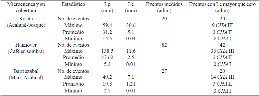
20, 82 and 27 events were analyzed for the micro-watersheds Rosita, Hannover and Berriozábal, respectively, processing data of precipitated sheet (Lp) and runoff depth (Le) measured at the output of each, with a Hellman type pluviograph and a type H flume with integrated limnograph, respectively. The disparity in the number of events analyzed respond to a couple of factors: (1) Of the three places, Hanover is the wettest and also has most of the events, and (2) Berriozábal is the farthest place from the largest populations and on a couple of occasions it was vandalized until finally the pluviograph was stole.

The Table 2 shows the statistical data of the events used to calculate the exposed Nc with field data for the three micro-watershed, using the expression 3. In this table, is noteworthy that, the Hannover site even though rain and runoff were measured in 84 events, only 42 showed runoff, which were those used to calculate Nc, as Equation 3 is only applicable when the runoff depth is higher than zero. Also in the Table 2, of the 42 events used of Hannover, 38 were in antecedent moisture condition (CHA) III; ie rain of the previous 5 days was higher than 50 mm.

Based on the Nc tables, reported by ^{McCuen (2004)} and ^{Campos (2002)} and also considering the type of soil, the hydrological conditions and the water group, the values of tables were determined corresponding to a NC₂ (CHAII and average slop of a a basin lower than 5%), for the three micro-watersheds. The carrying values are presented in Table 3.

Table 3 Definition of Nc₂ from the characteristics of the studied micro-watersheds. 

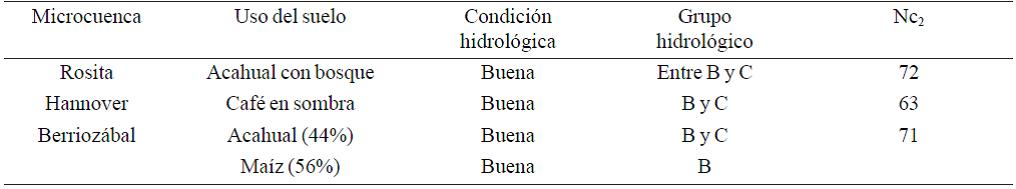
These values in Table 3 were subsequently corrected by slope and CHA with equations 8, 9 and 10, as corresponded and compared to the elect (estimated) tables. The comparison was made through the statistical called the relative error (ER%) calculated using equation 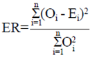11.

)11

Where: ER= relative error (%); O_i= observed value and, E₁= estimated value.

Results and discussion

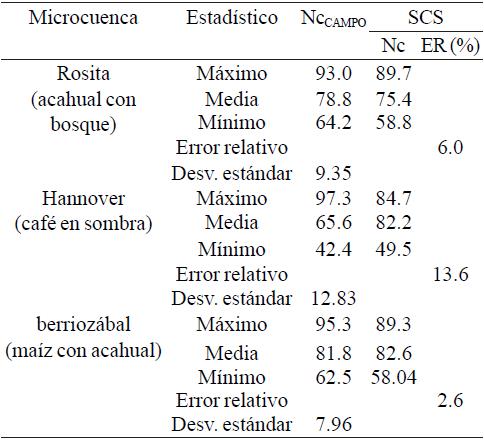
The Table 4 shows the range in which the values of Nc range, obtained with field data (Nc_field) and the estimated and corrected by slope and by CHA as was the case (Nc) for the three studied micro-watersheds. The relative error (ER) is also shown, by comparison between the Nc field and each of the estimated Nc; this comparison was by event. The biggest mistake was presented for the micro-basin Hannover, where there is more rain annually (with 5 175 mm in 2011) and the lowest error corresponds to the micro-watershed Berriozábal, which had the lowest rainfall in the same year (1 379 mm). It is also relevant to recall that in Hannover, of all the events used to calculate Nc, most of them were in CHA III; also in this micro-basin was detected the rain of the previous 5 days, taking values up to 531 mm (with an average of 196 mm), which is well above the threshold of 50 mm to declare it as CHA III of SCS.

Table 4 Comparison of runoff curves between calibrated in the field and the estimated corrected by slope and CHA. 

The Table 5 shows a summary of what might be Nc recommended in each micro-watershed for each CHA; although, it should be noted that for both Hannover and Berriozábal, the largest number of events are concentrated under the CHA III, and there are very few events with CHA I and CHA II. The micro-basin Rosita seems to have a different behaviour, since it is a place located in a populated area, at a lower elevation above sea level and where cattle usually graze; Rosita results contrast with those obtained by ^{Guichard et al. (2014)}, as they mention a higher value of Nc at 55. The differences may be due to ^{Guichard et al. (2014)} analizes not very accurate values, measured since 1955, in questionable located gauges, wich might imply that it did not even rain in Rosita. Besides, the data presented in this paper are updated, which considers the anthropogenic deterioration in watersheds, plus a texture, slope and antecedent moisture analysis.

Table 5 Summary of the average Nc for each antecedent hydrological conditions (CHA). 

*CHA I= condición seca; CHA II= condición media; CHA III= condición húmeda.

With respect to the moisture condition precedent, it must be clear that when Nc are used to design a hydraulic work or monitor an extreme event, it is recommended to use the data under a wet condition (CHAIII), under which it has a sample size more representative. But if what we want is to use the Nc for estimating runoff volume daily to carry monthly and then annually, it is simply recommend to use the average value of each site shown in Table 4.

According to ^{Hawkins (1993)}, the relationship precipitation per event, vesrus the number curve of runoffs can be of three types: complacent, standard or violent; being the most common standard and for which equations 2 and 4 are more applicable. The Figure 2 shows these relationships for the three micro-watersheds analyzed. The micro-watersheds Berriozábal and Hannover show a standard response behavior and, the micro-basin Rosita, even hough it seemed not to show a tendency towards one of the three patterns, usually (if the last two events are removed), the behavior is also standard.

Figure 2 Variation of the number of runoff curve according to precipitation. 

The equations shown in each of the graphs of Figure 2, shown only the trend of runoff curve in accordance with the classification of ^{Hawkins (1993)}: a) complacent behavior; b) standard behavior; c) violent behavior. These equations are suggesting not to be used for the number of runoffs curves, Nc. Since to determine an Nc is more complex than just making it dependent on rainfall, but rather are encouraged to consult the number of runoff curves contained in Table 5, which considers the Nc depends not only on what precipitates, but also texture, land-use and antecedent moisture condition.

Conclusions and recommendations

We recommend using the mean values of the number of runoff curve, obtained in this study and shown by Table 4, under the Nc_FIELD column, for calculating the daily runoff volume to carry it into monthly level, in those parts of the basins of the cost of Chiapas, where conditions of land-use and slope of the micro-watersheds under study (sandy-loam texture with acahual uses soil, forest, shade-grown coffee and maize; and with average gradient of basin at 25%).

On the coast of Chiapas, for the preparation of a design flood is recommended to use the values CHA III or wet in Table 5.

When values of Nc are used, from tables for the cost of Chiapas it is recommended to correct by slope, since a large percentage of their basins have sub-basins with average slope higher than 5%, except for the lower part of the basin, near the cities of Huixtla, Huehuetán and Tapachula; so to give examples of how little extension are in the coast Chiapas with slopes lower than or equal to 5%, for apply the value number of curve from the original tables of the late SCS from the US.

Future work is recommended in a more careful analysis of the antecedent moisture condition considering: (a) the clarifications made by ^{McCuen (2004)} for the growth and resting times and; (b) a new proposal of analysis for the CHA, as in cases like Hannover, rain of the previous 5 days is very high, and this site has the biggest error, resulting on an overestimated value of Nc when using SCS tables.