SciELO - Scientific Electronic Library Online

 
vol.14 número28Modelo matemático del aprendizaje acumulativo de un estudianteEfecto de la temperatura en la interacción entre Rhizopus stolonifer y Colletotrichum sp., patógenos de postcosecha en la yaca (Artocarpus heterophyllus Lam.) índice de autoresíndice de materiabúsqueda de artículos
Home Pagelista alfabética de revistas  

Servicios Personalizados

Revista

Articulo

Indicadores

Links relacionados

  • No hay artículos similaresSimilares en SciELO

Compartir


Nova scientia

versión On-line ISSN 2007-0705

Nova scientia vol.14 no.28 León may. 2022  Epub 01-Ago-2022

https://doi.org/10.21640/ns.v14i28.2723 

Natural sciences and engineering

Super-Twisting Control for trajectory tracking of a four-degree of freedom anthropomorphic robot manipulator

Control Super-Twisting para seguimiento de trayectoria en un robot manipulador antropomórfico de cuatro grados de libertad

Eddy Gabriel Ibarra1 

Yair Lozano Hernández1  🖂 
http://orcid.org/0000-0001-8157-3510

Manuel Alejandro Enríquez1 

Rosalba Galván Guerra2 
http://orcid.org/0000-0002-1945-2125

Mario César Maya3 

1 Instituto Politécnico Nacional. ESIME Zacatenco

2 Instituto Politécnico Nacional. UPIIH Hidalgo

3 Instituto Politécnico Nacional. CINVESTAV Zacatenco


Abstract

This work solves the regulation and tracking trajectories tasks for four degrees of freedom anthropomorphic robot manipulators. Two controllers are considered: a Super-Twisting controller (ST) and a Proportional Derivative with dynamics compensation (PD+) control. This comparison is carried out through numeric simulation of the dynamic model in the presence of disturbances using Matlab-Simulink software. Also, the tuning procedure of each controller is shown, as well as the stability criteria used for each case. The tunning of the ST controller is done considering the effects produced by an unknown Lipschitz disturbance; this guarantees robustness against this kind of disturbance. The results of the ST controller show the rejection of the disturbance, allowing the correct trajectory tracking. An algorithm based on the inverse kinematics solution is used to generate trajectories and their interpretation in generalized coordinates corresponding to the manipulator’s joint positions obtained through the geometric approach. In addition, we show the workspace, the manipulator parameterization, and the manipulator dynamic model through the Euler-Lagrange motion equations.

Keywords: motion control; sliding mode; anthropomorphic robot; manipulator robot; robustness; trajectory tracking; simulation; super-twisting; tuning; disturbances; algorithms; kinematics

Resumen

En el presente trabajo se resuelven las tareas de regulación y seguimiento de trayectorias para un robot manipulador antropomórfico de cuatro grados de libertad mediante un controlador Super-Twisting (ST), comparado con un control Proporcional Derivativo con compensación de la dinámica (PD+). La comparación se realiza mediante la simulación numérica en el software Matlab-Simulink del modelo dinámico con presencia de perturbaciones. También se muestra el procedimiento de sintonización de cada controlador, así como el criterio de estabilidad empleado para cada caso. Con respecto al controlador ST, la sintonización queda en función del efecto producido por una perturbación desconocida Lipschitz, lo que garantiza robustez a este tipo de perturbación. Los resultados del controlador ST muestran el rechazo de la perturbación, permitiendo el correcto seguimiento de trayectorias. En relación a la generación de trayectoria y su interpretación en coordenadas generalizadas correspondientes a las posiciones articulares del manipulador, se utiliza un algoritmo basado en la solución de la cinemática inversa, que se obtiene mediante enfoque geométrico. De igual modo, se muestra el modelo dinámico del manipulador a través de las ecuaciones de movimiento de Euler-Lagrange, el espacio de trabajo y la parametrización del manipulador.

Palabras clave: control de movimiento; modos deslizantes; robot antropomórfico; robot manipulador; robustez; seguimiento de trayectoria; simulación; super-twisting; sintonización; perturbaciones; algoritmos; cinemática

1. Introduction

The motion control of robot manipulators is a crucial task due to the wide range of applications in which such robots can be employed (Chua et al., 2003; Markert & Merk, 2009; Meike et al., 2013; Shepherd & Buchstab, 2014). In recent decades, various control algorithms have been used to address this problem, from the classic control to most recent approaches such as Fuzzy Control (FC), Neural Network-Based Control (NNBC), and Sliding Mode Control (SMC) (Arimoto, 1986; Orozco-Soto & Fernández, 2015; Lee & Choi, 2000). The classic control has proven its effectiveness in modern applications. For instance, in Román (2012) a Proportional Derivative (PD) control is designed to solve the regulation problem on a three degree of freedom (DOF) robot manipulator via brain waves, using a computer-brain interface. Another typical controller is the computed torque, a nonlinear controller based on the inverse dynamic model; such controller has been successfully implemented in many works and applications (Jaso & Rosas, 2015; Middletone & Goodwin, 1986; Park & Kim, 1998; Codourey, 1998). However, these techniques still carry some significant disadvantages in their design. For example, they do not consider the disturbance rejection in their structure. Besides, they tend to demand high gains in the control actions to have a good performance in the presence of disturbances.

Some modern control methods have been studied to develop and implement robust controllers in different robot manipulators, even without the need to know the system dynamic model. Such is the case of Meza (2003), where a fuzzy adaptive control based on observers is designed to identify and control nonlinear systems. For this method, the control actions are defined based on linguistic rules provided by an expert operator. However, although it would produce a reliable control law based on human experience, it could also be an inconvenience in the absence of such an expert (Sugeno & Takagi, 1993).

Sliding Mode Control (SMC) is an effective, robust nonlinear control technique (Shtessel et al., 2014; Sira-Ramírez, 2015) since it provides insensibility to coupled dynamics and robustness in the presence of disturbances. Therefore, its study has attracted attention in the field of robotics. In Piltan & Sulaiman (2012), a review of SMC in robotics shows recent attempts to implement SMC in robot manipulators. The main problem in using conventional SMC in electro-mechanical systems is the discontinuous nature of its control law, which produces actuator saturation, heat in mechanical parts, and the so-called chattering effect (Utkin et al., 2017). Several methods have been developed to attenuate or eliminate these effects in conventional SMC. Some exciting approaches include combining SMC with artificial intelligence techniques, producing hybrid variable-structure controllers focused on solving the motion control task in robot manipulators (Amer et al., 2011; Corradini et al., 2012; Vijay & Jena, 2017; Yu et al., 1999).

A different proposal is the use of the Second Order Sliding Mode Controllers (SOSMC). Within these control algorithms, we can find the Super-Twisting (ST) control, which was initially designed to be a continuous control law, capable of compensating smooth bounded perturbations (Levant, 1993; Levant, 1998; Moreno, 2009). This controller is widely used to replace discontinuous SMC with a continuous control law without losing robustness properties. Therefore, its use in robot manipulators has recently started to be explored (Trejo, 2018; Hernandez et al., 2011; González et al., 2007).

This paper aims to propose an ST controller capable of achieving an acceptable performance in trajectory tracking tasks for a 4 DOF robot manipulator, incorporating system robustness against parameter uncertainty, unmodeled dynamics, and external forces. Additionally, the stability conditions for the tuning procedure of the controller are presented. A PD with dynamic compensation (PD+) controller is designed for comparison purposes. A computational tool is used to test the performance of the proposed controllers in the trajectory tracking problem, and then the results are discussed and compared.

The remainder of the paper is organized as follows. Section two describes the problem for which we propose a solution. Section three describes the considerations taken into account about the manipulator configuration, along with the dynamic model of the system. Section four presents the structure of both control algorithms; in addition, the design and tuning procedure are detailed for each controller. In Section five, we exhibit the simulation results of each controller and present the discussion about them. Section six contains the conclusions derived from the realization of this work.

2. Methods, techniques, and instruments

Problem formulation

The motion control problem of robot manipulators carries several issues related to the effectiveness of the implemented controllers and the manipulator’s capability of executing some specific tasks. For instance, the efficacy of model-based controllers directly depends on the accuracy of the system model. However, in some cases, there may be discrepancies between such model and the physical system, mainly due to parameter uncertainty and unmodeled dynamics; these discrepancies may diminish the efficacy of these controllers. Furthermore, robot manipulators that operate away from controlled environments, such as the ones attached to explorer vehicles for space and deep-water missions, are usually submitted to unknown external forces, which affects the performance of the tasks assigned to the robot manipulator.

The described problems above can be treated as one if we group parameter uncertainty, unmodeled dynamics, and unknown external forces as a single perturbation term. This problem is known as disturbance rejection and can be addressed using a robust control strategy.

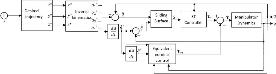
Therefore, the robust control strategy has relevance because it allows decreasing the effects of the mentioned features. Moreover, with this strategy, it is possible to obtain good performance for the robot manipulator tracking control problem. This work presents a solution for this issue through a sliding-mode-based control law known as ST controller. The methodology of the present work illustrated in Figure 1.

Figure 1 Solution methodology

Mathematical model

Let be the 4-joint robot manipulator shown in Figure 2a (without end-effector). Consider the coordinate frames fixed to the manipulator (see Figure 2b). The dynamic model is obtained using Lagrange’s equations, where the Lagrangian L(q,q˙) of a robot manipulator of 4 DOF is the difference between its kinetic energy K and its potential energy, U, That is:

Lq,q˙=Kq,q˙-U(q) (1)

Figure 2 (a) Virtual model of the manipulator; (b) Coordinate frames attached to the manipulator

Then the kinetic energy function K(q,q˙) and potential energy U(q) may be decomposed into the sum of four parts: Kq,q˙=K1q,q˙+K2q,q˙+K3q,q˙+K4q,q˙ and Uq=U1q+U2q+U3q+U4(q). Hence, using these equations, the Lagrangian is:

Lq,q˙=K1q,q˙+K2q,q˙+K3q,q˙+K4q,q˙-U1q-U2q-U3q-U4q. (2)

In addition, Rayleigh’s dissipation function is introduced into Euler-Lagrange’s dynamic equations, obtaining:

ddtq˙iLq,q˙-qiLq,q˙+q˙iRFq˙=τi,   for i=1,2,3,4. (3)

Where: RF=Bq˙2/2. Equation (3) corresponds to the manipulator dynamic equations, including the friction forces.

Thus, four dynamic equations correspond to the torques delivered by the actuators and can be expressed as follows:

τ=Mqq¨+Cq,q˙q˙+G(q)+Bq˙, (4)

Where: qRnx1 is the position vector, q˙Rnx1 corresponds to the velocity vector, BRnx1 is the vector that contains the viscous friction coefficients, q¨Rnx1 indicates the acceleration vector, MqRnxn is the symmetric positive definite manipulator inertia matrix (nonsingular and invertible), Cq,q˙Rnxn describes the centrifugal and Coriolis forces, G(q)Rnx1 is the vector of gravitational forces and τRnx1 represents the torque vector. The complete dynamic model is shown in Appendix A (Ibarra et al., 2019).

Manipulator parameterization

The control algorithm design requires the parameterization of the manipulator physical parameters used in the dynamic model. A manipulator design is made in the CAE-CAD SolidWorks software with the actual values of the structure dimensions and considering aluminum alloy 1060 as the primary construction material.

By using the virtual model of the manipulator, it is possible to analyze the physical properties of each of the links that make up the manipulator and thus obtain the parameters that describe it.

Considering that i is the ith link in the part of the manipulator structure that connects the joint (i+1) with the ith joint and separating the virtual model of the manipulator into four assemblies corresponding to the four links, each link of the manipulator is analyzed in SolidWorks as an independent assembly.

It is necessary to assign a new reference frame to each link based on the rules of Denavit Hartenberg’s method. The physical properties obtained are the total mass of each link, the entire length of each link, the center of mass of each link concerning the new reference frame, and the inertia tensor of each link to the new reference frame.

The viscous friction parameters which are present in the servo motors coupled to each joint are considered. Such friction values are obtained from a previous system identification made for the engines used in a manipulator with similar characteristics to the one studied in this work (Corke, 2017). The results of the parameterization performed are grouped in Table 1.

Table 1 Parameters of manipulator robot

Parameter Notation Value Units
Link length 1 L1 0.030 m
Link length 2 L2 0.124 m
Link length 3 L3 0.128 m
Link length 4 L4 0.160 m
Center of mass for Link 1 lc1 [0 -0.013 0] m
Center of mass for Link 2 lc2  [-0.056 0 0] m
Center of mass for Link 3 lc3 [-0.075 0 0] m
Center of mass for Link 4 lc4 [-0.104 0 0] m
Link mass 1 m1 0.069 kg
Link mass 2 m2 0.044 kg
Link mass 3 m3 0.097 kg
Link mass 4 m4 0.203 kg
Inertia tensor of link 1 I1 DiagIxx1, Iyy1, Izz1=Diag29560, 27115, 25219x10-9 kg.m2
Inertia tensor of link 2 I2 DiagIxx2, Iyy2, Izz2=Diag62147, 202246, 144735x10-9 kg.m2
Inertia tensor of link 3 I3 DiagIxx3, Iyy3, Izz3=Diag119639, 688704, 253732x10-9 kg.m2
Inertia tensor of link 4 I4 DiagIxx4, Iyy4, Izz4=Diag158281, 2577283, 2533430x10-9 kg.m2
Viscous friction coefficients B DiagB1,B2, B3, B4=Diag0.1668, 0.1668, 0.1668,0.1668x10-9 kg.m2s

The notation used in Table 1 is, centers of mass correspond to lci=x, y, z, which denotes the coordinate of the center of mass for the reference frame of each link. Also, the notation for the inertia tensor indicates a diagonal matrix, whose elements on the main diagonal correspond to the main moments of inertia Ixx, Iyy and Izz.

Control strategies

a. PD+ control

The PD+ Control for trajectory tracking is a robust passive computed torque controller (Han et al., 2020), which requires the exact knowledge of the manipulator’s dynamic model to be implemented (Kelly et al., 2006; Reyes, 2011), that is, of Mq, C(q,q˙), G(q) and B. In addition, it is necessary to know the desired trajectories q*t, q˙*(t) and q¨*(t) as well as to have the measurements q(t) and q˙(t). The PD+ is a globally stable controller that results from a Lyapunov function candidate Vt=1/2(q~˙TMqq~˙+q~Tkpq~), obtaining the following equation (see Slotine & Weiping (1988) for more information):

τ=τpd=kpq~+kvq~˙+Mqq¨*t+Cq,q˙q˙*t+Gq+Bq˙*t, (5)

Where: kp and kv are symmetric positive definite matrices, q~=q*t-q(t) denotes the position error and q~˙=q˙*t-q˙(t) the velocity error in the manipulator’s joints. For the application of the control law described in (5), it is necessary that Mq and Cq,q˙ are not independent, the matrix (M˙q-2Cq,q˙) must be skew-symmetric and that the dynamic structure is linear in terms of a suitably selected set of robot and load parameters (Slotine & Weiping, 1988; Han et al., 2020). Figure 3 shows the block diagram of the PD+ Control. For this case, we consider that we have access to all system information, compensating Mq,  Cq,q˙, Gq, and B.

Figure 3 Block-diagram of the PD+ Control

The gain tuning of the PD+ controller does not depend on the manipulator model nor the task assigned to it. It is usually suggested to be performed manually and based on the designer’s knowledge (Kelly et al., 2006; Reyes, 2011). To propose a tuning procedure for the PD+ controller, we assume that the control law compensates the nonlinear nature of the manipulator at some instant of time, then we can describe the manipulator dynamics of the form:

q¨=kpq~+kvq~˙. (6)

The linear system described in (6) is used for tuning purposes only and can be represented by the following block diagram:

Figure 4 Block diagram of the linear system

The closed-loop equation is:

qsq*s=kp+kvs2+kvs+kp . (7)

The selection of kp and kv must guarantee that the characteristic polynomial is Hurwitz. Therefore, we use the following reference model:

s2+2ζiωnis+ωni2=s2+kvis+kpi. (8)

Thus, kpi=ωni2 and kvi=2ζiωni,   for i=1,2,3,4. To have a low absorption energy behavior, the damping coefficients ζi=0.7 and undamped natural frequencies ωni=5.2, 4.8, 4, 3.5 are proposed. Then we group the gains in diagonal matrices as follows:

kp=diagkp1, kp2, kp3, kp4=diag27.04, 23.04, 16, 12.25, (9)

kv=diagkv1, kv2, kv3, kv4=diag7.28,  6.72,  5.6, 4.9. (10)

The controller gains, kp and kv, are positive definite symmetric matrices, this being a sufficient condition of stability (Kelly et al. 2006). Finally, Figure 5 shows the block diagram of the PD+ Control in closed-loop for path tracking.

Figure 5 Block diagram of the PD+ Control for path tracking

b. Control Super-Twisting control

Consider the existence of a Lipschitz disturbance term, the dynamic model of the robot manipulator is rewritten as:

q¨=Mq-1(τ-Cq,q˙q˙+Gq+Bq˙+Fq,q˙), (11)

Where: F(q,q˙) represents the perturbations/uncertainties vector produced by the disturbance force affecting the system, parameter uncertainties, and unmodeled dynamics. This term is assumed Lipschitz. To proceed with the design of an SMC law, we define the sliding surface as follows:

σt=q~˙+λq~,       with λ>0. (12)

The purpose of SMC is to force the sliding surface dynamics to reach the value of zero in a finite time and keep it at zero thereafter, i.e.:

σt=σ˙t=0. (13)

Once this is accomplished, the controlled dynamics are described by:

q~˙=-λq~. (14)

The solution of (14) is:

q~t=e-λtq~0, (15)

Thus, it is shown that the position error and its derivative converge to zero asymptotically. Deriving the sliding surface, we obtain:

σ˙t=q~¨+λq~˙, (16)

Where it is clear that: q~¨=q¨*-q¨, so (16) can be rewritten as:

σ˙(t)=q¨*-q¨+λq.~˙ (17)

Then, substituting (11) into (17), we have that:

σ˙t=q¨*+λq~˙-Mq-1(τ-Cq,q˙q˙+Gq+Bq˙+Fq,q˙). (18)

We propose the following control law:

τ=τeq+ueq, (19)

Where: τeq the equivalent nominal control, responsible for compensating the known system dynamics. Thus it is defined as follows:

τeq=Mqq¨*+λq~˙+Cq,q˙q˙+Gq+Bq˙. (20)

Thus, ueq must satisfy the condition σ˙t=0, substituting (20) in (18), we deduce:

ueq=-Fq,q˙. (21)

Equation (21) is the equivalent control and indicates that the second term of the control law should be equal to the negative of the disturbance term to assure the system’s robustness. However, this control action usually cannot be implemented, since it depends on the disturbance F(q,q˙) which is usually unknown (Shtessel et al., 2014).

To satisfy condition (13), the use of an SMC with the equivalent nominal Control is proposed, providing robustness to the system in the presence of disturbances. The proposed controller is a Super-Twisting (ST) control. Then the control law is rewritten as:

τ=τeq+τst, (22)

Where: τst is the ST control action defined as follows:

τst=Mqk1σt412+ω, (23)

ω˙=-k2signσt, (24)

With k1, k2>0 and σtn12=σt112signσt1, ,  σtn12signσtnT.

Figure 6 depicts the block diagram of the ST controller for the robot manipulator.

Figure 6 Block diagram of the STA controller

Substituting (22) in (18), we obtain:

σ˙t=-k1σtn12+ω+M(q)-1F(q,q˙) (25)

If Ω=ω+M(q)-1F(q,q˙), then (25) becomes:

σ˙t=-k1σtn12+Ω. (26)

Thus, Ω˙=-k2signσt+Mq-1F˙q,q˙+ddtMq-1F(q,q˙), proposing φ=Mq-1F˙q,q˙+ddtMq-1Fq,q˙ and φφMax=L. In this way, we obtain the following sliding surface:

σ˙t=-k1σtn12+Ω, (27)

Ω˙=-k2signσt+φ. (28)

At this point, the design problem is reduced to the setting of the parameters k1 and k2. In this work, we use the tuning rules for an ST controller proposed in (Levant, 1998), which indicates that:

k1=1.5L;    k2=1.1L. (29)

The stability proof for this tuning procedure is not developed in this paper. In exchange, we present sufficient conditions for the controller to be stable in finite time. In the interest of doing so, we use the stability proof for Super-Twisting parameter setting shown in Seeber & Horn (2017), from where we extract the following. Let us define the below system:

x˙1=-k1x112signx1+x2, (30)

x˙2=-k2signx1+δt, (31)

Where: δt is an absolutely continuous perturbation bounded by δtL.

Theorem 1: The system (30)-(31) is stable in finite time if its parameters satisfy the following conditions (Seeber & Horn, 2017).

k1>k2+L;    k2>L. (32)

Comparing (27) and (28) with (30) and (31), we can see that the sliding surface corresponds to the system form referred to in Theorem 1. Thus, such a theorem is valid to analyze the stability of the sliding surface. Observe that the parameter setting (29) proposed in (Levant, 1998) satisfy condition (32), which proves the finite-time stability of the ST controller with the use of these gains. Therefore, the sliding surface designed in this work is stable in a finite time by the following control law:

τ=Mqq¨*+λq˙*-λq˙+Cq,q˙q˙+Gq+Bq˙+Mqk1σtn12+ω, (33)

ω˙=-k2sign(σ(t)). (34)

To proceed with the setting of the gains k1 and k2, we estimate the bound L via the use of a Matlab-Simulink simulation environment. We propose an oscillatory perturbation with maximum perturbation torque of 1.5 Nm. The computed values were:

L=1800;   k1=63;     k2=1980. (35)

Finally, the design parameter λ was proposed to be λ=2.9.

Remark: Note that the proposed sliding mode controller is capable of compensating asymptotically Lipschitz uncertainties/perturbations. In the case of a discontinuity in the perturbation vector F, the controller will lose convergence, but after the discontinuity, it will reconverge if the derivative bound condition is fulfilled.

Inverse Kinematics

We use inverse kinematics to link the robot manipulator’s position and orientation in the workspace with the robot manipulator joint positions. In this paper, we decide to employ a geometric approach to obtain the inverse kinematics of the robot manipulator. Furthermore, we choose to restrict the inverse kinematic solution to the elbow-down solution.

Consider Figure 7, which represents the robot manipulator links and where the θi angles correspond to the angles formed by the robot manipulator links on each of the joints, with i=1,2,3,4. In addition, the angles formed by the second and third links are depicted in Figure 8. Furthermore, the F reference frame corresponds to the reference frame attached to the robot manipulator end effector.

Figure 7 Symbolic representation of the robot manipulator joints

Figure 8 Position relation formed by the linksa2anda3of the robot manipulator

The following homogenous transformation matrix denotes the position and orientation of the end effector:

H = RO01, (36)

Where: RR3x3 denotes the orientation matrix of the end effector and OR3x1 represents the origin point of the F reference frame.

From Figure 7 and equation (36), we define the position vector Oc as follows:

Oc=xcyczc=O-a4R100. (37)

Then, θ1 is derived from Figure 7 and equation (37) as follows:

θ1=atan2ycxc. (38)

From Figure 7 and Figure 8, we define the following parameters:

co=zc-d1, (39)

r=xc2+yc2, (40)

c2=r2+co2=a22+a32-2a2a3cosc^, (41)

Where: c^=180-θ3, and by trigonometric identities, we get:

cosc^=-cosθ3. (42)

Then, substituting equation (42) in equation (41), we obtain:

r2+co2=a22+a32+2a2a3cosθ3, (43)

From which we derived the following:

C3=cosθ3=r2+co2-a22-a322a2a3, (44)

S3=sinθ3=±1-C32. (45)

Then, θ3 is computed as follows:

θ3=atan2S3C3. (46)

Similarly, from Figure 8, θ2 is computed as follows:

α=atan2cor, (47)

β=atan2co2a2+ca=atan2a3S3a2+a3C3, (48)

θ2=α-β. (49)

Similarly, to compute θ4 we define the following:

ϕ=θ2+θ3, (50)

ϕ2=θ2+θ3+θ4, (51)

co3=H34-zc. (52)

Then, equation (51) is rewritten as:

ϕ2=asinco3a4. (53)

Finally, θ4 is derived as follows:

θ4=ϕ2- ϕ. (54)

Therefore, the solution to the inverse kinematics is defined by equations (38), (46), (49), and (54), which are grouped in a vector that denotes the actual joint positions of the robot manipulator given a homogenous transformation matrix for the robot manipulator end effector:

q=q1,q2,q3,q4T=θ1,θ2,θ3,θ4T. (55)

Robot task

The trajectory proposed in this work is intended to be smooth in time and be reachable by the end effector within the workspace of the robot manipulator. Such trajectory in the workspace is described by the following equations:

xt=0.04519t+0.325, (56)

yt=0.0219t-0.01, (57)

And finally, the variable zt is defined by a Bezier curve characterized by the following parameters: t1=0, t2=19, z0=0.066 and zf=0.066. Thus, these three variables are grouped in the following position vector:

dt=xt,yt,ztT, (58)

Which denotes the desired position of the robot manipulator end effector, and where the time variable t goes from 0 to 19 seconds. The total displacement of the trajectory in the workspace is depicted in Figure 9.

Figure 9 Desired trajectory in the workspace

The orientation of the robot end-effector can be defined in terms of the zf-axis of the robot end effector (see Figure 7). We define a variable named Yaw to denote the desired rotation angle for the robot end-effector. However, the orientation of the robot end-effector is constant at all times. Thus, Yaw is fixed as -0.3 rad, and the orientation of the robot end-effector is defined by the following rotation matrix:

RΨ=0.95530.2955000-1.0-0.29550.95530. (59)

Finally, we can group both, the position vector, and the rotation matrix in the following homogenous transformation matrix:

Hdt=RΨdt01. (60)

Thus, for each value of Hdt in time, a value for the vector qdt=qd1,qd2,qd3,qd4T is calculated using the inverse kinematics equations. Where qdt denotes the desired robot manipulator joint positions.

In summary, the robot’s end-effector must follow the trajectory and orientation described in (58). The inverse kinematics equations are thus used to find the necessary angles in each joint. Therefore, the reference values to be entered into the controller are obtained. Figure 10 shows the block diagram to get the desired angles for the robot’s joints.

Figure 10 Scheme used to know the desired angles in each joint. 

Numerical simulations

The designed control algorithms were tested in Matlab-Simulink, using the robot manipulator’s dynamic model to evaluate the performance of each controller for a trajectory tracking task. Such desired trajectory was designed to be smooth and differentiable in time.

As it was pointed out before, the perturbation term must be Lipschitz. Taking this into account, we propose Fq,q˙=-0.8cos2t+0.5q+0.2q˙Nm. The simulation fixed step time was set at 0.001s.

The performance of each control algorithm in both joint space, and workspace, for the trajectory tracking task in the presence of perturbations are shown in Figure 11 and Figure 12. From these figures, the PD+ Control is evidently more affected by the disturbance force than the Super-Twisting Control.

Figure 11 Trajectory tracking in joint space with PD+ Control

Figure 12 Trajectory tracking in joint space with ST

In addition, in Figure 13, we present the required torque by each controller. Note that the demanded torque by the Super-Twisting Control is a continuous function (see Figure 13b). Furthermore, it is essential to point out that part of the tunning criteria considers that the control outputs were bounded within a range corresponding to the actual value of torque given by commercial actuators.

Figure 13 (a) Control actions of PD+; (b) Control Control actions of ST control

3. Results and discussion

To provide an analytical analysis for the obtained results, we also include the position error achieved for each controller in both joint space and workspace. From Figure 14, we observe that the maximum error in the robot joint’s desired trajectory is bounded by 0.05 rad, which denotes the PD+ Control poor performance in the presence of perturbations. Meanwhile, in the case of the Super-Twisting controller, the position error is considerably smaller, being bounded by 1x10⁻⁴rad.

Figure 14 Position error in joint space with (a) PD+ Control; (b) ST Control

Additionally, we also include an error analysis for the joint space based on three error metrics named Incremental Error (IE), Incremental Absolute Error (IAE), and Mean Square Error (MSE), which are defined as follows:

IE = k=1Nq~i,k, (61)

IAE = k=1Nq~i,k, (62)

MSE =1N k=1Nq~i,k2, (63)

Where: N denotes the total number of samples, and i represents the joint number of the manipulator with i = 1,2,3,4. Figure 15 shows that the IE due to the PD + Control has an oscillatory behavior, while with the ST controller, the IE converges to a constant value. Similarly, Figures 16 and 17 show that the IAE and MSE due to the PD + controller tend to increase, while with the ST controller, they converge to a constant value.

Figure 15 IE (a) in robot joint 1; (b) robot joint 2; (c) robot joint 3, and (d) robot joint 4

Figure 16 IAE in (a) robot joint 1; (b) robot joint 2; (c) robot joint 3, and (d) robot joint 4

Figure 17 MSE in (a) robot joint 1; (b) robot joint 2; (c) robot joint 3, and (d) robot joint 4

Furthermore, from Table 2, we observe that the final value of IAE is significantly smaller for the Super-Twisting controller, up to 29 times smaller in joint one than its PD+ counterpart. Finally, the MSE value is lower with the Super-Twisting controller on most joints.

Table 2 Error Metrics (EM) obtained with PD+ and ST controllers [EM1,EM2,EM3,EM4]. 

EM PD+ Control Super-Twisting controller
IE -7x10⁻³,-7.61x10-2,0.528,-0.609 [1.1x10⁻²,-9.4x10-2,0.508,-0.598]
IAE [0.317, 0.434, 0.984, 1.181] [0.011, 0.095, 0.509, 0.599]
MSE [3.4x10-7,1.1x10-6,2x10-5,2.6x10-5] [9x10-9,6.8x10-7,1.9x10-5,2.2x10-5]

Bearing in mind that the ultimate goal of a robot manipulator is to execute an assigned task on its workspace, it is also essential to analyze Figure 18, from which we can see that the maximum position error achieved in the workspace by the PD+ Control in the presence of perturbations is bounded by 0.02m, the ST controller has a maximum position error of 4x10⁻⁵m. Indicating that the Super-Twisting controller is capable of executing higher accuracy tasks even in the presence of disturbances.

Figure 18 Position error in workspace with (a) PD+ Control; (b) ST Control

Furthermore, to illustrate Super-Twisting stability, the behavior of the sliding surface is shown in Figure 19. From such a graph, we observe that the sliding surface reaches the origin in a finite time and stays at zero thereafter, satisfying condition (13).

Figure 19 Sliding Surface

4. Conclusions

The present paper describes the development of a Super-Twisting controller applied to the motion control of a 4 DOF robot manipulator and its comparison with a classic PD+ control. From the obtained simulation results, we can state the following.

PD+ Control can solve the trajectory tracking problem. Nevertheless, its performance was affected by disturbances, which compromises the realization of the assigned task. Considering that the PD+ Control is a high gain controller, the disturbance rejection problem might be solved by increasing the controller gains until we obtain a complete disturbance compensation. Despite this may be seen as a possible solution, it could be conflicted with the physical limitations of the actuators.

On the other hand, from the position error plots, we can conclude that the Super-Twisting controller accomplished an adequate compensation of the disturbance term. Consequently, its performance was not diminished, making this controller suitable for high accuracy tasks even in the presence of perturbations. One main limitation of the SMC is the discontinuous nature of its control laws, which are usually hard to implement in electro-mechanical systems. However, as it was shown, in the case of the Super-Twisting, its control action is a continuous function. Therefore its physical implementation might be possible.

Furthermore, it should be noted that the actions of the ST control were limited to the actual value (same range as the PD +) of the commercial actuators torque, achieving an error (in the presence of disturbances) seven times less than the obtained with a PD +.

Currently, the problem of tracking trajectory in the presence of disturbances has been solved by various methods. However, our proposal shows in detail the stability conditions for the controller adjustment procedure. We use a Lipschitz-type function F(q,q˙) to analyze the unknown disturbances. As a result, we can guarantee that both the position error and its derivative converge to zero asymptotically. Though, if F(q,q˙) is not Lipschitz at some points; the controller will lose convergence. But, it will reconverge after the Lipschitz condition is satisfied again.

5. Supplementary information

Appendix.

6. Acknowledgements

The presented work was funded by Secretaría de Investigación y Posgrado del Instituto Politécnico Nacional (SIP-IPN), under the research grants 20210595, 20210709 and 20211316.

References

Amer, A. F., Sallam, E. A., & Elawady, W. M. (2011). Adaptive fuzzy sliding mode control using supervisory fuzzy Control for 3 DOF planar robot manipulators. Applied Soft Computing, 11(8), 4943-4953. [ Links ]

Arimoto, S. (1986). Stability and robustness of PD feedback control with gravity compensation for robot manipulator. Robotics: Theory and Applications-DSC, 3, 67-72. [ Links ]

Chua, P. Y., Ilschner, T., & Caldwell, D. G. (2003). Robotic manipulation of food products-a review. Industrial Robot, 30(4), 345-354. https://doi.org/10.1108/01439910310479612 [ Links ]

Codourey, A. (1998). Dynamic modeling of parallel robots for computed-torque control implementation. The International Journal of Robotics Research, 17(12), 1325-1336. https://doi.org/10.1177%2F027836499801701205 [ Links ]

Corke, P. (2017).Robotics, vision and Control: fundamental algorithms in MATLAB® second, completely revised(Vol. 118). Springer. [ Links ]

Corradini, M. L., Fossi, V., Giantomassi, A., Ippoliti, G., Longhi, S., & Orlando, G. (2012). Minimal resource allocating networks for discrete time sliding mode control of robotic manipulators. IEEE Transactions on Industrial Informatics, 8(4), 733-745. [ Links ]

González Rodríguez, A., Pineda Ortega, M., & Soberanes Leal, D. M. (2007). Seguimiento adaptativo de trayectorias con convergencia en tiempo finito de un robot antropomórfico virtual de tres grados de libertad. [Tesis para obtener el grado de Licenciado en Ciencias Computacionales. UAEH]. http://dgsa.uaeh.edu.mx:8080/bibliotecadigital/bitstream/handle/231104/163/robot%20antropomorfico%20virtual.pdf?sequence=1&isAllowed=yLinks ]

Han, S., Wang, H., Tian, Y., & Christov, N. (2020). Time-delay estimation based computed torque control with robust adaptive RBF neural network compensator for a rehabilitation exoskeleton. ISA transactions, 97, 171-181. [ Links ]

Hernandez, D., Yu, W., & Moreno-Armendariz, M. A. (2011). Neural PD control with second-order sliding mode compensation for robot manipulators. In The 2011 International Joint Conference on Neural Networks (pp. 2395-2402). IEEE. [ Links ]

Ibarra, E. G., Enriquez, M. A., Lozano, Y., Galván-Guerra, R., & Maya, M. C. (2019). Modelado cinemático y dinámico de un manipulador antropomórfico de cuatro grados de libertad. Pädi Boletín Científico de Ciencias Básicas e Ingenierías del ICBI, 7(Especial), 116-123. [ Links ]

Jaso, A. & Rosas, D. I. (2015). Brazo robótico planar con dos grados de libertad. [Ingeniería en Comunicaciones y Electrónica. Instituto Politécnico Nacional, Escuela Superior de Ingeniería Mecánica y Eléctrica]. [ Links ]

Kelly, R., Davila, V. S., & Perez, J. A. L. (2006). Control of robot manipulators in joint space. Springer Science & Business Media. [ Links ]

Lee, M., & Choi, H. S. (2000). A robust neural controller for underwater robot manipulators. IEEE Transactions on Neural Networks, 11(6), 1465-1470. https://doi.org/10.1109/72.883478 [ Links ]

Levant, A. (1993). Sliding order and sliding accuracy in sliding mode control. International Journal of Control, 58(6), 1247-1263. [ Links ]

Levant, A. (1998). Robust exact differentiation via sliding mode technique. Automatica, 34(3), 379-384. [ Links ]

Markert, J., & Merk, G. (2009). U.S. Patent No. 7,603,927. Washington, DC: U.S. Patent and Trademark Office. [ Links ]

Meike, D., Pellicciari, M., & Berselli, G. (2013). Energy efficient use of multirobot production lines in the automotive industry: Detailed system modeling and optimization. IEEE Transactions on Automation Science and Engineering, 11(3), 798-809. [ Links ]

Meza, A. (2003). Observadores difusos y control adaptable difuso basado en observadores. Centro de Investigación y de Estudios Avanzados del Instituto Politécnico Nacional. [ Links ]

Middletone, R. H., & Goodwin, G. C. (1986). Adaptive computed torque control for rigid link manipulators. In 1986 25th IEEE Conference on Decision and Control (pp. 68-73). IEEE. [ Links ]

Moreno, J. A. (2009). A linear framework for the robust stability analysis of a generalized super-twisting algorithm. In2009 6th International Conference on Electrical Engineering, Computing Science and Automatic Control (CCE)(pp. 1-6). IEEE. [ Links ]

Orozco-Soto, S. M., & Fernández, J. C. R. (2015). Control par calculado difuso basado en pasividad para seguimiento de trayectorias de robots manipuladores. Research in Computing Science, 91, 131-141. [ Links ]

Park, J. H., & Kim, K. D. (1998). Biped robot walking using gravity-compensated inverted pendulum mode and computed torque control. In Proceedings. 1998 IEEE International Conference on Robotics and Automation (Cat. No. 98CH36146) (Vol. 4, pp. 3528-3533). IEEE. [ Links ]

Piltan, F., & Sulaiman, N. B. (2012). Review of sliding mode control of robotic manipulator. World Applied Sciences Journal, 18(12), 1855-1869. [ Links ]

Reyes Cortes, F. (2011). Robótica: control de robots manipuladores (No. 004.896 629,892). [ Links ]

Román, M. A. (2012). Control de un robot manipulador mediante la interpretación de ondas cerebrales. [Maestría en Tecnología de Cómputo. Instituto Politécnico Nacional, Centro de Innovación y Desarrollo Tecnológico en Cómputo]. https://tesis.ipn.mx/handle/123456789/21508?show=fullLinks ]

Seeber, R., & Horn, M. (2017). Stability proof for a well-established super-twisting parameter setting. Automatica, 84, 241-243. [ Links ]

Shepherd, S., & Buchstab, A. (2014). Kuka robots on-site. In Robotic Fabrication in Architecture, Art and Design 2014 (pp. 373-380). Springer, Cham. [ Links ]

Shtessel, Y., Edwards, C., Fridman, L., & Levant, A. (2014).Sliding mode control and observation. Springer New York. https://link.springer.com/book/10.1007/978-0-8176-4893-0 [ Links ]

Sira-Ramírez, H. (2015).Sliding mode control: the delta-sigma modulation approach. Birkhäuser. [ Links ]

Slotine, J. J., & Weiping, L. (1988). Adaptive manipulator control: A case study. IEEE transactions on automatic Control, 33(11), 995-1003. [ Links ]

Sugeno, M., & Takagi, T. (1993). Fuzzy identification of systems and its applications to modelling and Control. Readings in Fuzzy Sets for Intelligent Systems, 15(1), 387-403. [ Links ]

Trejo Zúñiga, E. C. (2018). Estudios de controladores por modos deslizantes de orden superior en robots manipuladores. [Maestría en Ciencias en Sistemas Digitales. Instituto Politécnico Nacional]. https://tesis.ipn.mx/bitstream/handle/123456789/26210/Trejo%20Z%c3%ba%c3%b1iga%2c%20Elmer%20C%c3%a9sar_DP.pdf?sequence=1&isAllowed=yLinks ]

Utkin, V., Guldner, J., & Shi, J. (2017).Sliding mode control in electro-mechanical systems. CRC press. [ Links ]

Vijay, M., & Jena, D. (2017). PSO based neuro fuzzy sliding mode control for a robot manipulator. Journal of Electrical Systems and Information Technology, 4(1), 243-256. https://doi.org/10.1016/j.jesit.2016.08.006 [ Links ]

Yu, W., Poznyak, A. S., & Sanchez, E. N. (1999). Neural adaptive Control of two-link manipulator with sliding mode compensation. In Proceedings 1999 IEEE International Conference on Robotics and Automation (Cat. No. 99CH36288C) (Vol. 4, pp. 3122-3127). IEEE. [ Links ]

Received: October 24, 2021; Accepted: June 04, 2021

🖂 Correspondence author: ylozanoh@ipn.mx

Contribution of the authors in the development of the work

The authors declare that they contributed equally.

Interest conflict

The authors declare that there is no conflict of interest.

Creative Commons License This is an open-access article distributed under the terms of the Creative Commons Attribution License