


 nueva página del texto (beta)
 Inglés (pdf)
 Artículo en XML
 Referencias del artículo
 Enviar artículo por email
 Citado por SciELO
  Similares en
SciELO
Similares en
SciELO 
 Permalink
Introduction
Diabetes mellitus is a chronic degenerative disease that is characterized by high blood glucose levels. This disease occurs when the pancreas stops producing insulin, when it does not produce it in enough quantities, or when the organism cannot use the insulin properly. Lack of insulin produces high glucose levels in the blood. This phenomenon is known as hyperglycemia and can severely damage many of the body's systems, e.g., cardiovascular, and nervous, in the long term (Wilmot et al., 2012). Consequently, a group of metabolic diseases like cardiovascular diseases, neuropathy, nephropathy, retinopathy, and blindness might follow a diabetes diagnosis. By controlling the blood glucose levels, some of these diseases might be prevented or delayed (Harris et al., 1987).
Diabetes is diagnosed by testing blood glucose levels (World Health Organization [WHO], 2016). If one or more of the following criteria are satisfied: 1) the fasting blood glucose level is larger or equal to 126mg/dl 2) blood glucose is present after two hours of ingesting 75g of glucose 3) the blood glucose taken at random is larger than 200mg/dl.
Many diabetes patients periodically monitor their glucose levels, and they use insulin shots to compensate for the pancreas insulin production insufficiency. These patients might benefit from tools that help them decide when to apply insulin (Amaris et al., 2017). The use of a predictive algorithm might be beneficial in these cases, and if the historical glucose levels follow a pattern, then their future values might be anticipated. For example, in reference (Zhao et al., 2012), a prediction of glucose levels from continuous monitoring data is made using autoregressive models with exogenous inputs that establish the future glucose levels as a lineal combination of current and recent glucose levels. In that reference, an laten variable based technique is used to develop an empirical model for predicting the patient's glucose levels.
The glucose levels are known for their instability and nonlinearity. For example, Frandes et al. (2017) modeled the glucose dynamics using nonlinear chaotic properties by monitoring the glucose levels in patients under free-living conditions; autoregressive models were applied to predict glucose levels in 30- and 60-minutes time intervals. The logistic smooth transition autoregressive model obtained a high precision for high glucose variability patients.
Panella (2011) demonstrated that neural networks are useful to approximate a function from their inputs using previous data in the time series. Gaussian neural networks can be used efficiently to predict type 2 diabetes's temporal evolution by considering the biologic time series's chaotic nature.
Ståhl and Johansson (2009) showed how to estimate quantitative predictive models to design optimal insulin levels for the patients. Three aspects were considered: 1) insulin, 2) glucose, 3) insulin-glucose interaction, and different black-box and gray-box models were developed and analyzed. The models' short-term predictors for the glucose levels were designed to achieve prediction within two hours.
The neural networks (NN), multi-rate regression, and autoregressive integrated moving average (ARIMA) models are the most used models to study the evolution and make predictions. In Velásquez et al. (2008), nonlinear models are used to predict the monthly electricity demand. Among these models, the multilayer perceptron, the autoregressive neural network (ARNN), and the ARIMA model were compared to predict the monthly electricity demand in Colombia by using only the demand's historical data. ARNN showed less percentage of error, while in (Amaris et al., 2017).
Tang et. al. (1991) compared three different times series with different characteristics and the they concluded that for time series with long memory both ARIMA and NN performed similarly, while for short memory the NN appeared to be superior. In contrast, for prediction of the solar radiation, Reikard (2009) concluded that ARIMA was superior. In another study (Adamowski et al., 2012) compared several linear and nonlinear regression, ARIMA, NN and wavelet NN for urban water demand forecasting concluding that the wavelet NN was superior.
In this work, an analysis of the fasting glucose level is done to predict the following five values, comparing the ARNN and ARIMA models. The ARNN takes advantage of autoregressive (AR) models and multilayer perceptron (MLP) to capture glucose levels' complex dynamics. The ARIMA models are composed of three elements: autoregressive models (AR), an integrator (I), and the mobile averages (MA), which are useful to find longitudinal data adjustments.
Several experiments with ARNN were performed using three different configurations by modifying the number of neurons. The obtained results show that ARNN were favorable as compared against the ARIMA model. The two-layer and ten-neurons ARRN showed that 73% of the signals obtained error percentages below 25%.
Method
The data used in this work was obtained from the Diabetes-Data database, composed of 70 patients' data providing information like dates, glucose level monitoring times, and insulin dosages, along with aliment consumption and exercise performed (Michael, 2017).
The ARIMA and ARNN models describe one or more variables over time. These models have been applied to predicting currency exchange rates, rainfall levels, and energy consumption. The artificial neural networks allow emulating the processing of information that the brain performs and allow it to be approximated to any function (Velásquez et al., 2008). The ARRN combines an autoregressive linear model (AR) and multilayer perceptron (MLP) that contains a hidden layer. The ARNN is a model that allows using the advantages of the AR and MLP to capture complex dynamics (Velásquez et al., 2008; Velásquez et al., 2009). The architecture of an ARNN is shown in Fig. 1.
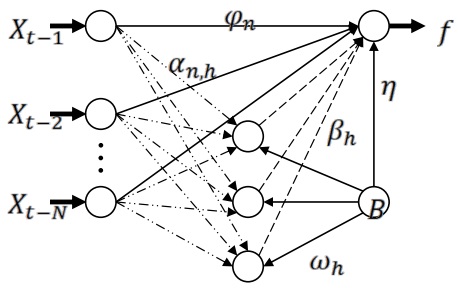
The ARNN model has a dependent variable f, that is obtained from applying a nonlinear function to N previous values, Xt-n for n = 1,…,N:
Where:
Where GG is the sigmoid adaptive function define as:
The model parameters are
Box developed statistical models for the time series (Box et al., 1994), where each observation value is modeled as a function of previous values (Amaris et al., 2017; Velásquez et al., 2008; Breu et al., 2011; Casdagli, 1989; Broz and Viego, 2014). These models are known as ARIMA and are composed of the following parts: 1) autoregressive (AR) 2) integrand (I) 3) moving average (MA), this in order to adjust the longitudinal data.
The ARIMA models predict the future values of time series based on historical behavior, without considering the underlying factors responsible for the variations of the dependent variable (Broz and Viego, 2014). The ARIMA workflow is shown in Fig. 2; the process starts by identifying the candidate model for the series to evaluate, following by an estimation, which refers to selecting the appropriate data. Next, a validation stage takes place, and the process ends with the prediction of future values.

The p, d, q, values must be assigned appropriately to model the time series's behavior and then select a reduced set of models to try to adjust the series. The ARIMA model is composed of 3 values (p, d, q), p represents the value of the autoregressive component (AR), d corresponds to the order of the integrand component (I), and q is the order value of the moving averages (MA).
ARIMA models can be expressed as:
Where:
φ is the autoregressive coefficient
θ moving average coefficient
ε error
Yt-1Yt-1 normalized series value
The neural networks (NN) have been used for the prediction in time series. A common error is not to realize that there is not an accepted methodology by the scientific community, but a set of guidelines and critical steps that have been adapted from general heuristics, the researcher ability, and previous knowledge of the analyzed series (Velásquez et al., 2008; Zhang et al., 1998).
Results
A series of tests were performed based on the literature review. The models were applied to the 70 subjects in the available database in order to compare their performance. Each series has N glucose level samples; 70% of the data was used for training, and 30% for the prediction validation. Each one of these series has a different behavior since each of the individuals has a different lifestyle. In Fig. 3, three different signals are shown. The signals shown in Fig. 4 show glucose levels above 120 mg/dl.

Each, the ARIMA and ARNN models were applied to the elements of the database. In the ARIMA model, the signals were used in weekly cycles that showed the best results. The quantity of data available to each series is reduced with the number of cycles to find, train, and approximate the expected values.
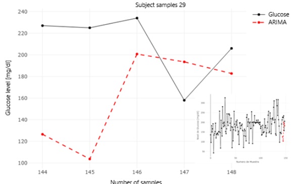
Fig. 4 and Fig. 5 show the signals from subjects 29 and 56. Zooming in the region of interest is also shown along with the predicted values using ARIMA. In those plots, it can be observed that the expected and predicted values are close to each other.

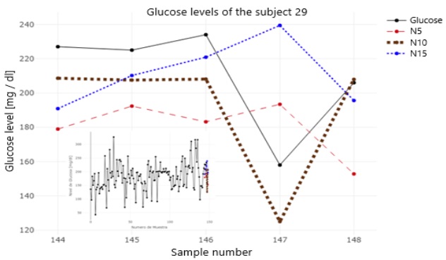
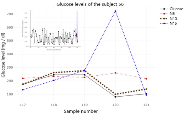
The ARNN was applied to each of the available times series using three different configurations, in Fig. 6 and 7, the predicted values for each of the configurations used by the ARRN. The five-neurons configuration is marked in red, in green the ten-neurons configuration, and the fifteen-neurons configuration was plotted in blue.
An evaluation of the results obtained using the two different prediction models was performed. As metrics, the absolute error (AE), mean squared error (MSE), and the root mean square error (RMSE) were used. Those results are presented in this section to predict the five subsequent values of the glucose levels. Table 1 shows the average error values by prediction of each of the tests performed.
Table 1 Percentage of average error (%).
| Prediction Number | |||||||
|---|---|---|---|---|---|---|---|
| MAE | 1st | 2nd | 3rd | 4th | 5th | Total | |
| ARIMA | 99.79 | 80.85 | 90.09 | 75.61 | 93.11 | 87.89 | |
| ARNN (5) | 64.60 | 57.15 | 68.16 | 63.26 | 65.27 | 63.69 | |
| ARNN (10) | 28.07 | 33.18 | 32.44 | 24.90 | 34.68 | 30.65 | |
| ARNN (15) | 70.58 | 60.90 | 54.58 | 67.58 | 83.46 | 67.42 | |
| MSE | ARIMA | 14696.77 | 12006.81 | 12959.12 | 10385.84 | 13557.66 | 12721.24 |
| ARNN (5) | 7353.49 | 6757.86 | 9324.24 | 8523.18 | 7449.15 | 7881.58 | |
| ARNN (10) | 1831.04 | 2510.09 | 2678.64 | 1320.53 | 2773.57 | 2222.77 | |
| ARNN (15) | 9945.59 | 9462.17 | 6018.96 | 14076.87 | 21935.19 | 12287.76 | |
| RMSE | ARIMA | 121.23 | 109.57 | 113.83 | 101.91 | 116.43 | 12721.24 |
| ARNN (5) | 85.75 | 82.20 | 96.56 | 92.32 | 86.30 | 88.77 | |
| ARNN (10) | 42.79 | 50.101 | 51.756 | 36.33 | 52.66 | 47.14 | |
| ARNN (15) | 99.72 | 97.274 | 77.582 | 118.64 | 148.10 | 12287.76 | |
It should be noted that after performing the evaluations on the 70 patients with the four proposed models, the calculation of the mean absolute error (MAE), the mean square error (MSE), and the root of the mean square error (RMSE) by prediction and by the model was performed. It was identified that 73% of the 70 subjects evaluated obtained error percentages lower than 25% in the MAE with ten-neurons in the ARNN. However, the other 27% of the evaluated subjects obtained errors between 39 and 156, being the more accurate model. Since the glucose levels are known for their instability and nonlinearity, most of the literature on the subjects tries to predict the glucose in the short term (Ståhl, 2009), using time series with sampled data in intervals from 5 to 120 minutes, see for example Table 1 in (Hameed, 2020), or in other cases using continuous information (Pérez-Gandía, 2010). The data that we have available has samples of approximately 24 hours, however this is the data that is available to the DM patients since they typically measure their sugar before breakfast.
The results obtained with the ARIMA model were not close enough to the sampled glucose values. The prediction values were high. In particular, when comparing with the values obtained by the ARNN.
Linear regression is applied between the expected value and the predicted value; a line at 45 degrees' angle will represent a high precision in the predictions, it is possible to observe the scatterplots that show the positive linear correlation between the sampled glucose levels and each of the model's predictions. In Fig. 8, the ten-neurons ARNN model is the model that approximates the most to a 45% degrees' straight line. It can also have observed that the data dispersion is less than in the other models; thus, this is the best model in our evaluation. It is also possible to infer from our data that the ARIMA model is not appropriate to predict glucose levels, or at least not when using univariate time series.
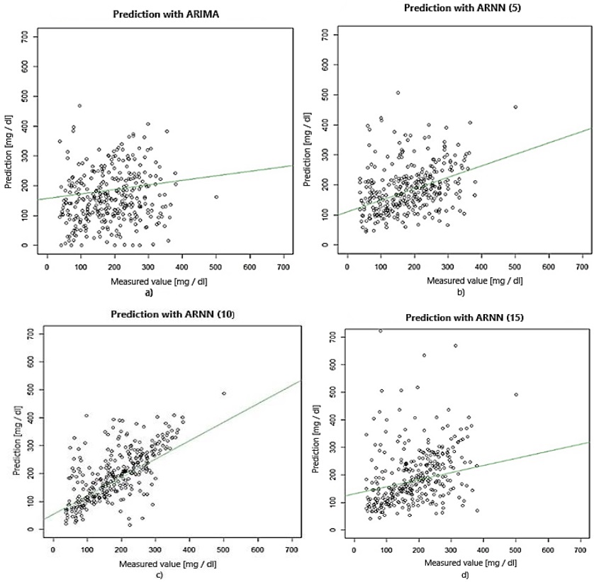
Fig. 8 Glucose sampled value and a) ARIMA, b) ARNN with 5 neurons, c) ARNN with ten-neuronss, d) ARNN with 15 neurons.
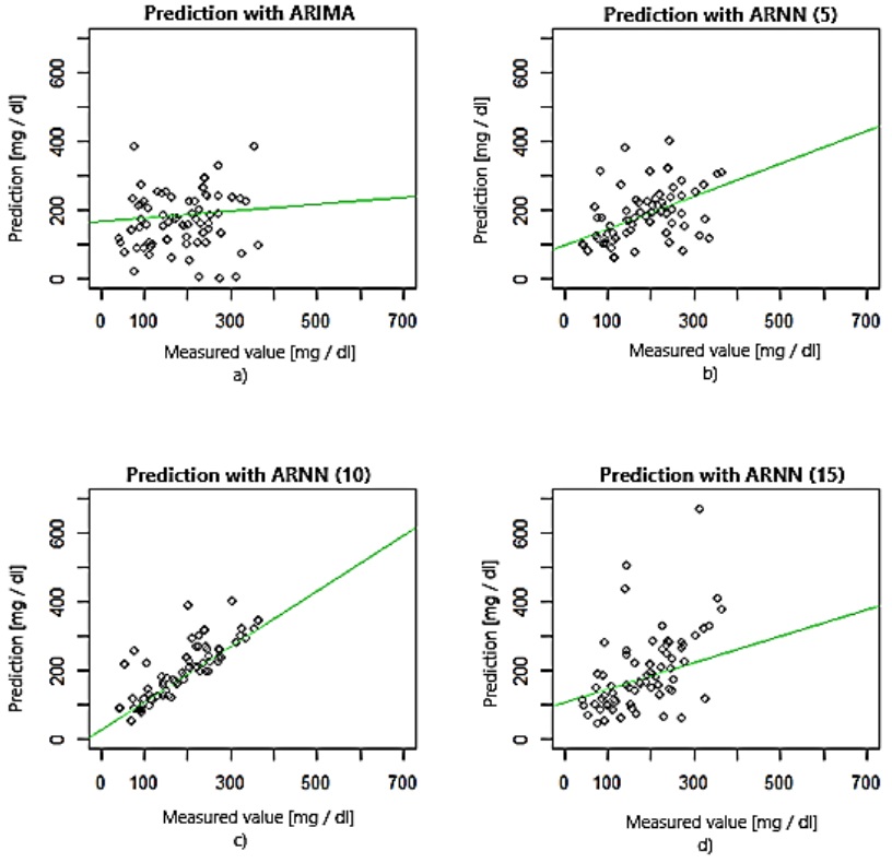
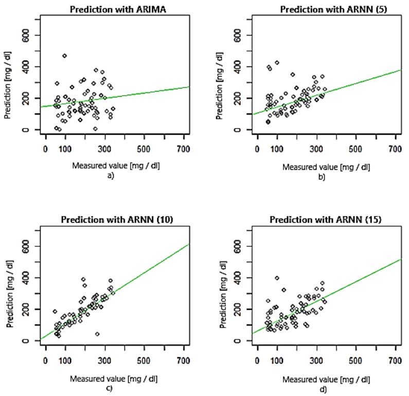
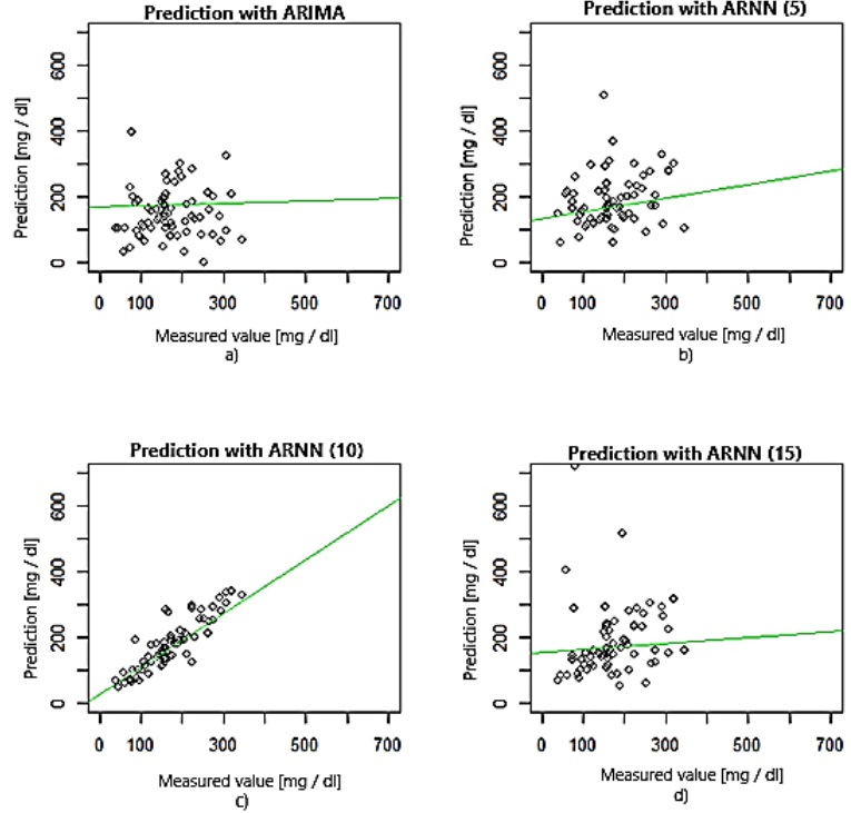
To compare the performance of each model, a linear regression analysis was performed for each model and to the five predicted values. The scatterplots and the linear adjustment for the first, second, third, fourth, and fifth predictions can be observed in Fig. 9, 10, 11, 12, and 13, respectively.


The R-squared adjustment is a statistical tool to measure how well a model predicts the sampled data; in other words, it is a measure of the relation between the predicting and goal variable. The R-squared takes values between 0 and 1; if close to zero the regression does not explain the variance in the response. On the other hand, a number close to 1 explains well the variance in the observed value in the output. In Table 2 are listed the obtained values for the R-squared of each prediction.
Table 2 coefficient of determination.
| Prediction number | |||||
|---|---|---|---|---|---|
| 1st | 2nd | 3rd | 4th | 5th | |
| ARIMA | 0.03489 | 0.004939 | 0.0156 | 0.0128 | 0.006496 |
| ARNN (5) | 0.272 | 0.1769 | 0.09595 | 0.03649 | 0.1266 |
| ARNN (10) | 0.8007 | 0.658 | 0.6876 | 0.7695 | 0.6613 |
| ARNN (15) | 0.1545 | 0.2783 | 0.3203 | 0.002408 | 0.001855 |
In Fig. 9, it can be observed that the first prediction of the ARIMA model underperforms. However, the ten-neurons ARNN model approaches better the expected value; this is evident when comparing their respective values of the coefficient of determination since the first prediction for the ARIMA has a value of 0.03489, which is close to 0, and the ten-neurons ARRN has a value of 0.8007 which approaches 1.
In Fig. 10 it can be observed that the models follow the same trend. The R-Squared for the second prediction in the ARIMA model is 0.004939, while for the ten-neurons ARNN has a value of 0.658.
In Fig. 11, 12 and 13 the scatterplots of the third, fourth and fifth predictions are shown. The R-squared value is 0.0156, 0.0128, and 0.006496, respectively for the ARIMA model and 0.6876, 0.7695 and 0.6613, for the ten-neurons ARNN.
Based on the results obtained and analyzing the linear regressions and r-squared, the ARIMA model is not adequate for predicting glucose levels since the values for both tests were close to 0, indicating that there is no reasonable relation between the predicted and target variables values. In the ARNN model, the results obtained with the regressions are very favorable. It is verified with the R-squared adjustment values, which in the 5 predictions are the closest to 1, which indicates that the linear relationship between both variables is good. It should be noted that the first and fourth predictions of the ARNN model with ten-neurons are those that are closest to the predicted values.
In the ARNN model with fifteen-neurons, predictions four and five are not reliable since their R-squared adjustment is very close to 0. In deciding to use this model to predict glucose levels, it is crucial to consider that the prediction would be sufficient for three values ahead. However, the best model for predicting glucose levels is the ARNN model with ten-neurons. It is the model that its average absolute error by prediction and in general are the lowest. In terms of the R-squared adjustment, it is the model that finds the best relationship between the prediction and the target variable.
Conclusion
The performance of the ARIMA and ARNN model for the prediction of glucose levels was analyzed. The results show that ARNN can predict up to five values of glucose. In 73% of the cases, the error was below 25%. On the other hand, the ARIMA model shows that only 6% of the cases had an error below 25%. It is important to mention that a prediction will never be completely accurate since many variables related to each patient's behavior are not considered and cannot be controlled. Despite that, we have established that ARNN is a viable option based on the relative and absolute errors for prediction and as a whole for glucose prediction. The ARNN was also the model that obtained the best R-squared adjustment to the predicted and sampled values. As future work, we would like to include categorical data into our database to classify the patients according to meat consumption, physical activity, insulin dosage, and sampling time.

