


 nueva página del texto (beta)
 Inglés (pdf)
 Artículo en XML
 Referencias del artículo
 Enviar artículo por email
 Citado por SciELO
  Similares en
SciELO
Similares en
SciELO 
 Permalink
Introduction
The World Health Organization (WHO) mentioned that in the next years, blindness and others visual limitation diseases would become one of the world's leading socio-economic problems and it could slow down the advance of many developing countries 1. More than 300 million of people in the world live with visual disability, due to eye diseases. Of those people, 45 million are blind and 90% live in low socio-economic countries. The main causes of blindness are cataracts (39%), uncorrected refractive errors (18%), glaucoma (10%), age-related macular degeneration (7%), corneal opacity (4 %), diabetic retinopathy (4%) between others 1.
According to data from the National Institute of Statistics and Geography (INEGI) in Mexico it is estimated that 5.1% of the Mexican population have some disability, and 27.2% of them are visual disabilities. INEGI ties these numbers to the population age and indicates that most of this population is concentrated in the adult age groups that could be economically active 1. Based on the motivation to decrease this tendency, there is a growing attention on the research fields focused on diagnose visual pathologies in an early stage, when the disease is still treatable. Many research trends have been developed in last decades, one of them centered on the extraction of electrical activity of the optic nerve (O.N.) from the occipital EEG signal registered during a session where the patient is exposed to a sequence of external visual stimulus. The electrical activity of the O.N., that is the object of interest in this work consist in a well characterized waveform composed by several peaks that appears around approximately 100ms after given stimulus and it is called visual evoked potential (VEP). Usually, VEP signal is hidden by high level of noisy signal (0<SNR<5)22 mainly electrical noise 3, that could be composed by the register of other kind of cerebral activity. One of the major concerns in this research field is to retrieve the VEP in a reliable way and avoiding interference from denoising methods that can affect latency.
In this paper, a comparative analysis between different techniques to detect and to separate the VEP from the simulated EEG signal is presented. Techniques were assessed quantitatively assuming a healthy case. The aim is to define an effective method to detect and separate the VEP from the EEG signal for its future application on glaucoma diagnosis. It is achieved performing the required analysis and processing to the EEG signal to extract only the characteristic waveform corresponding to the VEP by means of external periodic stimulation.
Visual evoked potential as a diagnostic indicator
The most common techniques applied to clinically assessing physiological aspects of the visual pathway are tonometry, campimetry and diagnostic imaging techniques, such as retinography and optical coherence tomography (OCT). All them are the essential tools for a diagnosis and control of pathologies, nevertheless studies had shown that patients can lose until 40% of their ganglion cells in the retina (RGC) before visual defects can be detected by these techniques. Standard Automated Perimetry (SAP) is the current gold standard for assessing visual function in patients with partial visual loss, like glaucoma patients 2.
Therefore, researchers are developing for new technologies, techniques that help them identify reliably and accurately the early loss of glaucomatous in the visual field. Research suggests that certain subpopulations of RGC are damaged in early glaucoma 2. This article describes VEP, as a technique that reviews these special cells.
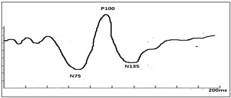
The VEP is a type of electroencephalographic signal (Fig. 1) and it is also the electrical response of the occipital cortex caused by visual stimulations through 23,24:
VEPs assess the function and integrity of the visual pathway from the photoreceptors (especially in the central area) to the occipital cortex, through bipolar cells and ganglion cells 24. They quantify the functional integrity of optical pathways better than scanning techniques, such as magnetic resonance imaging (MRI) 3,7,24.
Any abnormality that affects the visual pathways or the visual cortex in the brain can affect the VEP wave 4,5,6, 7 in the following parameters (Fig. 2):
Amplitude: Attenuation of the regular amplitude is present due to visual affection.
Latency: it is defined as the period between stimulus and the corresponding VEP occurrence instant. A delay on latency can be present on a disease condition.
Waveform (severe damage): the amplitude waves is too small and is difficult to find it because the characteristic form of the VEP is lost.
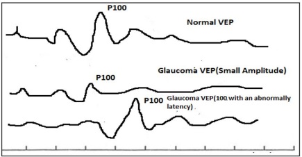
In Fig. 2, normal VEP waveform is illustrated, followed by two abnormal VEP waveforms: the first one affected in amplitude and the second one in latency.
Theory about techniques to extract VEP
In order to obtain the VEP signal, the following steps must be followed 7,9,11:
Wave identification (NPN form it occurs close to 100ms after a stimulus).
Determine the latency of absolute peaks.
Determine the amplitudes of the waves.
Determine the difference between latencies of both eyes.
In routine clinical studies, three peaks are normally identified: the first one with a latency of 70ms as negative peak (n70), followed by a positive peak with a latency of 100ms (p100) and finally a negative peak with a latency of 135ms (n135). The p100, or first positivity that occurs in latency around 100ms, is the most constant and useful in the clinical study. It is considered the most persistent and reliable peak 7,8,23.
P100 is generated in the area of the pre-striated cortex of the occipital lobes. Its average latency varies between 89 and 114ms with an amplitude of 3-21uV and a range of maximum difference (on latencies) between the two eyes of 6msec (Table 1).
Table 1 Variable parameters in VEP 6.
| Parameter | Value for a typical P100 |
|---|---|
| Latency | 89-114ms |
| Amplitude | 3-21uV |
| Normal difference between latencies of both eyes | 6ms |
Assessment of visual field damage has been performed analyzing the different parameters of VEP. In this sense, the first challenge is the reliable extraction of VEP waveform from EEG signal. The amplitude of the VEP signal is between 4 and 20μV 3,5,6. It is less than the amplitude of the undesirable components coming from electrical noise, Electromyographic (EMG) signal and Electrooculographic (EOG) signal, which are mixed in the EEG signal burying the VEP waveform. Different techniques have been developing to reach this aim.
To detect glaucoma disease, first it is necessary to clean the signal. Some authors have been used the average techniques to get the VEP as a traditional technique 10,8,12, but the problem lies that a big number of signals is necessary to increase the SNR of the average data that it’s translated in a long session that can tire out to the patients.
Other papers propose new techniques as FFT filter before averaging, or adaptative filters 8,12 to reduce the session time with less signals. Traditional VEP extraction method is the superposition averaging technique 12,18.
Also, there are some VEP extraction methods using neural network (NNA), wavelet transform 18, support vector machine (SVM) 20, blind source separation (BSS) 19)(21. Typical applied filters are: IIR-Chebyshev I, IIR-Chebyshev II, Elliptic, FIR Equirrible, FIR Least Square band pass between 5-48Hz 13, using windowing segment of 200ms 8.
Method
Fig. 3 present a scheme of the methodology. The objective was to assess the performance of different processing techniques used to extract VEP waveform from the EEG signal. The first stage was to segment the EEG signal using five distinct kinds of windows. The standard technique to process the signal is the averaging in which each recorded signal is windowed, this requires at least a rectangular window, each segment contains a hidden VEP. The rectangular window with a narrow main lobe has excellent resolution characteristic for comparable strength signals with similar frequencies, but it is a poor choice for noise suppression. Flat top window has low side lobe peak, which does not provide a high frequency resolution but can measure the strength of a signal accurately at any frequency. Between the extremes, some moderate windows, such as Hamming and Hann, are used commonly as a tradeoff among narrow main lobe (corresponding to high frequency resolution), low side lobe peak and rapidly fall-off side lobes(corresponding to noise suppression)26. In this paper different windows were used to segment signals: rectangular, nuttall, Hamming, Flattop, and Chebyshev, to observe its impact on the efficiency of certain noise suppression method for VEP extraction purpose.

Once signals were windowed, each segment was denoised. In this stage, nine different options were evaluated: the first one without filtering, the following four based on IIR filters (Butterworth, Chebyshev, Elliptic, and Bessel filters), and the last four based on wavelets (Daubechies 4, Simlets 4, Biorthogonal 2.6 and Coiflets 2). At the end of this stage, segments were classified as results of a certain windowed - denoised combination 14.
Finally, windowed and denoised segments of each combination were averaged (3600 epochs for 6Hz, 4800 for 8Hz and 5400 for 9Hz) to obtain a final VEP waveform. The number of segments was chosen in based of the size recorded signal, the common window size for VEP and the time where the waveforms appear in a normal VEP. No information about published standard for the number of segments neither size of window was found, nevertheless a range between 1 and 14 minutes for EEG signal acquisition has been reported 6,8,9. In total, 45 final VEP waveforms were obtained (it results from 5 windowing classes and 9 denoising techniques).
To perform a quantitative assessment of techniques, the following parameters were computed from the resulted final VEP waveforms: signal to noise ratio (SNR), mean square error (MSE), average latency (AL), latency standard deviation (LSD), and latency coefficient of variation (LCV).
As it was described above, to maintain rigorous controlled conditions for technique assessments, a set of synthetical VEP signals was simulated based on a typical VEP waveform. In the next section, the afore mentioned procedure is described.
Signal simulation
Two sets of ten signals were synthetized. Each set represents the VEP signals obtained from ten subjects during a session of 10 minutes of visual stimulus 3,13. A sampling frequency of 1000 Hz was considered because it allows to measure delays of the P100 peak latency in the order of milliseconds. One set of signals considers a constant latency of 100 ms, another set consider a random latency (with a media of 100 ms and a standard deviation of 10 ms). A simple model was used to simulate the VEP signal. Due that the main problem in this kind of signals is the interference or electronic noise from electronic device 25, in the simulation, as an approach to real signals whole of them were corrupted with additive white noise. The algorithms of simulation were developed in MATLAB software.
A synthetic VEP signal (Fig. 4c) was generated from a convolution of a basic waveform (sine wave) (Fig. 4a) and pulse train function (Fig. 4b) with different frequencies (6, 8, and 9 Hz). The sine wave shape was used to emulate the characteristic behavior of the NPN peaks. These are representative peaks of the VEP.
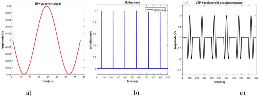
Once the artificial signals were generated, these were contaminated with additive white noise (Fig. 5a). It was obtained from a normal distribution using a standard deviation of 1mV (Fig. 5b).

Case 1: Synthetic signals with constant latency
Simulated VEP signals with an amplitude of 1μV and a constant latency of 100 ms between the stimulus and P100 peak were created as an ideal signal with the aim to assess the changes in the latency of the signals by the applied processing techniques. Three frequencies were considered in the simulation of stimulus, 6 Hz, 8 Hz, and 9 Hz.
Case 2: Synthetic signals with random latency
Random latency was computed from a Gaussian distribution with AL of 100 ms and LSD of 10 ms. This case represents a more realistic situation, where the VEP latency is not constant but (in healthy case) it can vary in the range between 89 and 114 ms. The used value of LSD was based on references that specify the variation of the latency in the traditional VEP (Table 1)6. In this case, also, the signals were generated with an amplitude of 1μV and at frequecies of 6 Hz, 8Hz, and 9Hz.
Generation of noisy signals
All the synthetic simulated signals were corrupted with additive white noise generated from a normal distribution using a standard deviation of 1mV.
Signal processing methods
All the simulated signals were segmented using five kinds of window with a size of 200 ms. These were rectangular, nuttall (4-term Blackman-Harris window), Hamming, symmetric flat top, and Chebyshev. The size was chosen because the important VEP response waveform occurs between 70 and 150 ms after the stimulus was presented 23,24.
Another stage of the signal processing was the filtering. Nine alternatives were probed: coherent average, four digital filters (Butterworth, Chebyshev, Elliptic and Bessel), and four families of wavelets (Daubechies 4, Simlets 4, Coiflets 2, and Biorthogonal 2.6) 17.
In the case of the coherent average and digital filters methods, these were applied to all signals, i.e. simulated signals with constant latency and with random latency. The used parameters for the digital filters are showed in Table 2.
Table 2 Filter parameters.
| Filter type | Band pass [Hz] |
|---|---|
| Butterworth | 4 to 40 |
| Chebyshev I | 4 to 40 |
| Elliptic | 4 to 40 |
| Bessel | Down to 40 |
Using the signals with constant latency the performance of the processing techniques was tested with the aim to choose a combination of window plus digital filter that could identify a VEP. A resulted combination based on digital filter was used to process the simulated signals with random latency. In all cases, after the signal segmentation procedure, using the mean of the whole of segments, the latency of the P100 peak was computed.
For the wavelet denoising, the hard thresholding was applied, and a four level of decomposition was used. This denoising method was applied to simulated VEP signals of 10 minutes of duration with random latency. Then, the signal segmentation procedure was applied, and the mean of all segments was obtained. For each window, the latency of the P100 peak was computed.
To assess the performance of the methods (windowing plus denoising techniques) the SNR, the MSE between the original signal (without noise) and the processed signal, the AL of the P100 wave, the LSD, and the LCV were used.
Assessing parameters
The parameters used to assess the signal processing methods were the SNR, the MSE, and the latency of the P100 wave. The SNR was computed using (1). This parameter measures the quality of the signal with respect to the noise. Thus, a system, which enhance a signal (high SNR) is better because the signals are less influenced by noise.
Where: PPS is the processed signal power, and OSP is the original signal power.
The mean square error (MSE) is defined in (2) and it is used to compare the original signal and the processed signal. It gives a measure of similitude between signals therefore two identical signals will have and MSE value equal to zero.
Where: n is the length of the signal,
The LSD parameter (σ) was computed from (3) 15:
Where: n is the number of samples,
xi
is the signal, and
Where: n is the number of subjects,
xi is the
i-subject latency, and
The LCV indicates the variability of a set of latencies independently of the used units. It is defined in (4)16).
Where: σ is the standard deviation, and
Results
In this section, simulated signals are shown; also results of performed evaluations are presented in three phases: I) obtained from applying windowing- IIR denoising techniques to signals of case 1; II) obtained from applying the same techniques of previous case to signals of case 2; and III) obtained from applying windowing - wavelet denoising techniques to signals of case 2. Assessed parameters obtained from the 45 final VEPs were compared and analyzed.
Simulated Signals
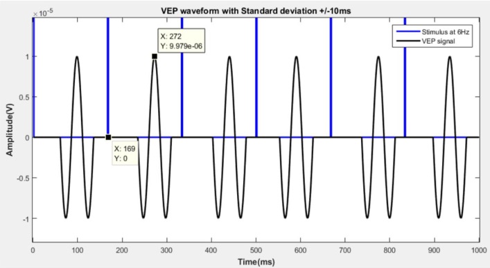
As it was described above, two kinds of signals were simulated: The called “Case 1” with a constant latency value of 100 ms and the second case (Case 2) with a random latency value centered in 100 ms and with a standard deviation (SD) of 10 ms. In Figs. 6 and 7, simulated signal corresponding to 6 Hz is illustrated. It represents the “original” signal, before to be added with simulated noise. It is possible to appreciate two kinds of waveforms: the blue one, composed by a periodic series of spikes corresponds to the stimulus signal; it means that each spike indicates the instant of stimulus occurrence. This waveform is depicted just with illustrative purposes. The black signal corresponds to the set of VEPs based on the characteristic waveform composed by the three peaks: N75, P100 and N135. The first case is depicted on Fig. 6, it is shown that each VEP is located exactly 100 ms after stimulus occurrence (constant latency). In the graph, some tags indicating instants of stimulus and VEP occurrences have been added to illustrate the constant latency. The second case is graphed on Fig. 7, the random latency can be appreciated. As in the previous case, tags were inserted, and variable latency is observed. Finally, on Fig. 5, a signal with added noise is presented.

Fig. 6 The blue line represents the stimulus every 6Hz and the black line represent the VEP response.
Results of Signal processing
In Fig. 8a, graphs corresponding of different stages of the signal processing are shown. A segment of signal containing a VEP is shown. The segment of original simulated signal is marked in black, then the same segment with added noise is graphed with magenta color line. The blue line waveform is the windowed segment (using a Chebyshev window) and finally the N averaged segments without filter applied are illustrated with red line. Due the small amplitude of the original signal and the average signal they are showed in Fig. 8b.

Fig. 8 a) Processing of the VEP signals contaminated signal, original simulated signal, windowing segment, and average for the case 1. b) Average and original VEP signal.
Other two cases are presented in Figs. 9 and 10. The first one (Fig. 9a) corresponds to stages of signal processing using a rectangular window and an elliptic filter applied to a synthetic signal with random latency. The segment of original simulated signal is marked in black, then the same segment with added noise is graphed with magenta color line. The blue line waveform is the windowed segment (using a rectangular window) and finally the N averaged segments without filter applied are illustrated with red line. Due the small amplitude of the original signal and the average signal they are showed in Fig. 9b.

Fig. 9 a) Processing of the VEP (with standard deviation of +/-10) signals contaminated signal, original simulated signal, windowing segment, and average for the case 2. b) Average and original VEP signal.
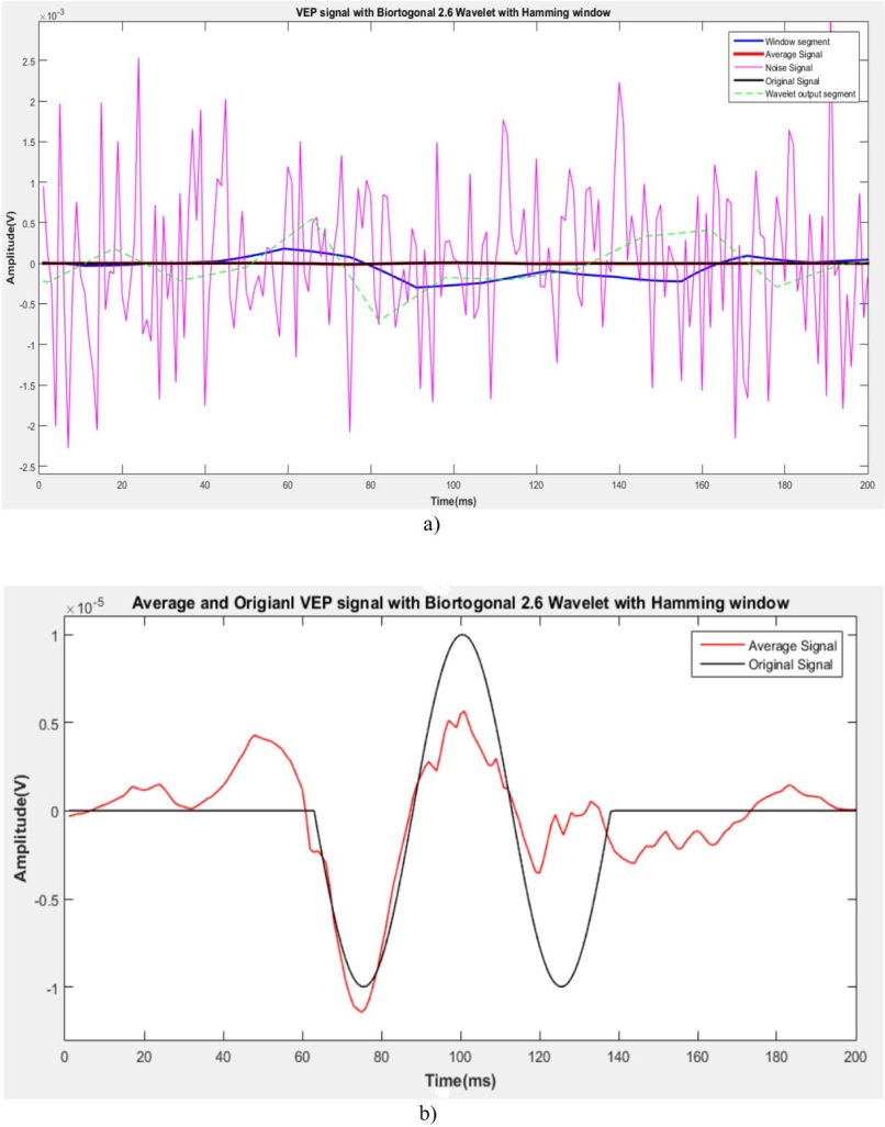
The second (Fig. 10a) represents stages of signal processing considering denoising by means of the wavelet Biorthogonal 2.6 and a Hamming windowing. The segment of original simulated signal is marked in black, then the same segment with added noise is graphed with magenta color line. The blue line waveform is the windowed segment (using a Hamming window), the N averaged segments applied are illustrated with red line and finally the output Wavelet filter is the green dash liner. Due the small amplitude of the original signal and the average signal they are showed in Fig. 10b.
Results of evaluation
Methods applied to signals with constant latency
In Fig. 11, results obtained of the parameters of interest evaluated in the case of signals with a constant latency: SNR, MSE and AL are presented in different graphs(a-c). Each graph is composed by 25 data (per frequency), which are distributed in the following way: the first five points of each graph correspond to the five window functions without filter applied, the second set of five points corresponds to the five window functions with the Butterworth filter, the third set represents five window functions for the Chebyshev filter, the fourth set for the Elliptic Filter and the fifth set for the Bessel filter. For major clarity, in Table 3 are listed the configuration followed to present data illustrated in Fig. 11 and Fig. 12.
Table 3 “X” axis description for Figs. 11 and 12.
| x Label | Filter Type | Window function | x Label | Filter Type | Window function |
|---|---|---|---|---|---|
| 1 | Without filter | Rectangular | 16 | Elliptic Filter | Rectangular |
| 2 | Nutall | 17 | Nutall | ||
| 3 | Hamming | 18 | Hamming | ||
| 4 | Flattop | 19 | Flattop | ||
| 5 | Chebyshev | 20 | Chebyshev | ||
| 6 | Butterworth Filter | Rectangular | 21 | Bessel Filter | Rectangular |
| 7 | Nutall | 22 | Nutall | ||
| 7 | Hamming | 23 | Hamming | ||
| 9 | Flattop | 24 | Flattop | ||
| 10 | Chebyshev | 25 | Chebyshev | ||
| 11 | Chebyshev Filter | Rectangular | |||
| 12 | Nutall | ||||
| 13 | Hamming | ||||
| 14 | Flattop | ||||
| 15 | Chebyshev | ||||

Fig. 11 Results of the assessment performed to signals with constant latency. a) AL; b) SNR; and c) MSE values for each windowing-denoising method are presented. The three cases are reported: when the stimulus was generated at 6 Hz (blue line), at 8 Hz (orange line) and at 9 Hz (gray line).
A graph for each parameter is shown as in the “x” axes the numbers represent the type of window function and the filter type as show the Table 3.
The parameters were obtained for each subject and then an average of the 10 subjects for each specific windowing-denoising combination was obtained. Resulted averages were analyzed to find the best results.
It is clearly appreciated that the best results of AL (Fig. 11a) were obtained with the method without applied filter, due to in this case of constant latency, its value of 100 ms was almost kept by all windowing methods: 110.9 ms -101.04 ms for 6 Hz, 100.84 ms -101.04 ms for 8 Hz an 100.94 ms-101.01 ms for 9Hz.
The Butterworth filter also obtained good results, and among the windowing methods, the Nuttall window obtained an AL value of 102.34 ms for 6 Hz, 101.78 ms for 8 Hz and 101.43 ms for 9 Hz, overcoming those results obtained without filter. Elliptic, Chevy and Bessel filters did not achieve results approximated to the original latency of 100 ms in any case.
About SNR (Fig. 11b), the Elliptic filter option reached the best values, followed by the non-filter specifically for the case of 6 Hz. The other methods presented small values of SNR.
The methods behaviour regards MSE (Fig. 11c) was similar: the smallest values of MSE (the best options) were achieved by Bessel filter and Elliptic filter options, followed in this case by non-filter option. The other methods obtained higher values for MSE.
Methods applied to signals with random latency
Techniques based on digital filters. As it was mentioned in methodology, the techniques based on digital filters were also applied to signals with random latency. In Fig. 12, results obtained of the parameters of interest evaluated in the case of signals with a random latency: SNR, MSE, LSD, LCV and AL are presented in different graphs, from a) to e), for the three frequencies. A graph for each parameter is shown following the same configuration for data presentation used in the previous section (as listed in Table 3)
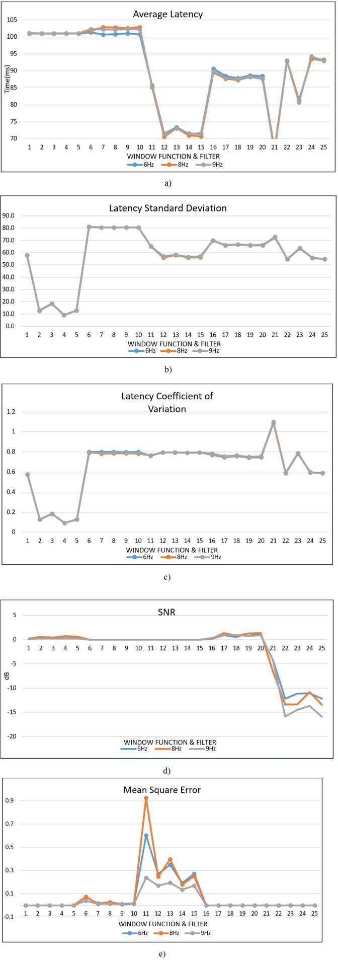
Fig. 12 Results of the assessment performed to signals with random latency. a) AL; b) LSD; c) LCV; d) SNR; and e) MSE values for each windowing-denoising method based on digital filters are presented. The three cases are reported: when the stimulus was generated at 6 Hz (blue line), at 8 Hz (orange line) and at 9 Hz (gray line).
It is clearly appreciated that the best results of AL (Fig. 12a) were obtained with the method without applied filter, followed by the Butterworth filter option. For the case of non-applied filter, AL values were kept near to 100 ms for all windowing methods: 100.9-101.005 ms for 6 Hz, 100.91-101.05 ms for 8 Hz an 100.99-101.11 ms for 9Hz.
The LSD obtained data (Fig. 12b) showed that the best result was obtained with a non-filter with flattop window for all frequencies, 9.13 ms for 6Hz, 9.11 ms for 8Hz and 9.09 ms for 9Hz and the worst case was obtained with the Butterword filter with rectangular window option: 81.01 ms for 6Hz, 80.98 ms for 8Hz and 90.99 ms for 9Hz. Regard, the LCV (Fig. 12c) the smallest values correspond to those obtained by means of non-applied filter option combined with the flap top window (0.09 for 6 Hz, 8 Hz and 9 Hz).
In Fig. 12d, results for SNR are illustrated; the best option was the elliptic filter with Flattop window with a value of 1.25 dB. The worst case was the Bessel filter with Chebyshev window with a value of -12.78 dB.
Finally, MSE (Fig. 12e) show that elliptic and Bessel filters got the minimum values for this parameter, followed by the non-filter techniques. The best combination was for Bessel filter with flattop window.
Techniques based on wavelets. In this section, results obtained by means of denoising methods based on different kinds of wavelets are presented. As in the previous case, parameters of interest: SNR, MSE, AL, LSD and LCV are depicted (Fig. 13). In Table 4, the data configuration per graph is specified.

Fig. 13 Results of the assessment performed to signals with random latency with a variation of +/-10ms. a) AL; b) LSD; c) LCV; d) SNR; and e) MSE, AL and LSD values for each windowing-denoising method based on wavelets are presented. The three cases are reported: when the stimulus was generated at 6 Hz (blue line), at 8 Hz (orange line) and at 9 Hz (gray line).
Table 4 “X” axis description for Fig. 13.
| x Label | Wavelet function | Window function | x Label | Wavelet function | Window function |
|---|---|---|---|---|---|
| 1 | Daubechis 4 | Rectangular | 11 | Biortogonal 2.6 | Rectangular |
| 2 | Nutall | 12 | Nutall | ||
| 3 | Hamming | 13 | Hamming | ||
| 4 | Flattop | 14 | Flattop | ||
| 5 | Chebyshev | 15 | Chebyshev | ||
| 6 | Symlets 4 | Rectangular | 16 | Coiflets 2 | Rectangular |
| 7 | Nutall | 17 | Nutall | ||
| 7 | Hamming | 18 | Hamming | ||
| 9 | Flattop | 19 | Flattop | ||
| 10 | Chebyshev | 20 | Chebyshev |
Regard AL values(Fig. 13a), the Simlets 4 wavelet reached the most approximated results to reference value (100 ms) for all windowing methods and for the three cases: 6, 8 and 9 Hz; among them, the best results were obtained for the Simlets 4 with rectangular function window. However, all wavelet methods achieved AL values between 100.115 ms and 101.18ms.
The LSD (Fig. 13b) obtained values with all wavelets were bigger than those obtained with the non-filter option of the previous case (and the gold standard technique used in this field), all the standard deviation values fall above 15 ms whereas the gold standard method presents values near to 10 ms (with almost all kinds of windows). For wavelet analysis, the increment of the frequency (form 6 Hz to 9 Hz) was did not affected results, they keep similar values on most of the wavelet function and, however in all the worst cases where a was observed for rectangular window was applied (and independently of the used wavelet), the standard deviation was closed to 60 ms.
The LCV data (Fig. 13c) were similar than those obtained with the non-filter option. The LCV values for wavelets methods fell between 60% (0.602) and 18% (0.18), and for the non-filter option (with any kind of window) values were in a range between 60 and 15% (0.6 - 0.15).
SNR (Fig. 13d) results were, in general, better to that obtained with non-filter option. SNR values for the cases of wavelets varies within a range between 1.64 - 7.43 dB, whereas the SNR values for the non-filter option (considering the five windowing options) varies between 0.1 to 0.6 dB. The best results for the three frequencies were those obtained by the Coiflets 2 - Flat top window. The worst results were with the rectangular window function in all wavelet.
An interesting observation in the MSE (Fig. 13e) results is that the best estimations were obtained by the Flattop window, independently of the kind of used wavelet. In general, all the MSE results estimated with wavelets (that fell in a range between 1.2e-6 ms - 3.8e-6 ms) were slightly lower to that obtained with the non-filter option (5.8e-6 ms - 16.57e-6 ms).
Discussion or Conclusion
There is a wide range of assessment parameters referenced in bibliography used to evaluate method of VEP extraction performance, i.e. SNR, peak amplitude, eccentricity, the number of false positives, latency variation, etc. In this paper, five parameters were proposed: SNR, MSE, AL, LSD, and LCV as representative factors to be considered on evaluations of VEP extraction methods. SNR and MSE were focused to assess the level of noise that remain in signal after windowing & denoising method was applied. In the other hand AL, LSD and LCV were oriented to evaluate the impact of the method on the VEP latency estimation.
The gold standard method used as a traditional tool of extracting VEP waveform is the VEP segments averaging in which the segmentation is performed using a rectangular window for each segment. Usually, VEP segments are obtained from a windowing process of raw EEG signal. Few information about performance of windowing and denoising techniques applied to improve the averaging method are available for this reason, in this work different windowing function are evaluated as mentioned before. In this work, an evaluation of digital filters and wavelets denoising techniques was performed with the aim to find a combination of windowing and denoising technique that might improve the traditional technique performance. For the analysis of wavelet denoising technique the performance of several wavelet function (combined with different kind of windows) was assessed the option with best results was identified. For all the wavelet techniques that were assessed, the P100 was the most important wave to identify assuming that the NPN waveform is preserved in all simulated cases. In a future work, cases considering a distortion of the NPN waveform could be analyzed considering a wider variety of wavelet functions in order to define performance of this kind of denoising methods to detect a distorted VEP. Assessment results obtained in this work showed that for the ideal signal (constant latency), the best digital filter technique was the based on Butterworth filter, that independently of the window type its results were similar to those obtained for the traditional method of averaging without any filter option. The best SNR results were reached by the elliptic filter technique follow by the non-filter option. The smaller MSE values were obtained by means of Bessel and Elliptic filters as well as by the averaging technique similar for both options. Butterworth filter also obtains small values of MSE. The Chebyshev filter in general, presented the worst results in all parameters.
A slight performance degradation on AL results obtained with Butterworth filter option (and independently of window method) were detected when signals with random latency were processed, LSD and LCV values obtained with all filters were higher than those ones obtained with the traditional method. Regards SNR and MSE, filter behavior kept similar to the case of constant latency: all filters approximate values obtained with the traditional method (average method) except the Chebyshev filter for MSE values and the Bessel filter for the SNR values
Finally, denoised methods based on different kinds of wavelets were evaluated. In this case the option that achieved the best results of AL, LSD and LCV was the ones based on Biorthogonal 2.6 and the Coiflets 2 wavelets, specifically combined with a flattop window, providing excellent approximated values to reference values, similar to like the traditional case and improving SNR MSE values when rectangular this window was used.

