


 nueva página del texto (beta)
 Inglés (pdf)
 Artículo en XML
 Referencias del artículo
 Enviar artículo por email
 Citado por SciELO
  Similares en
SciELO
Similares en
SciELO 
 Permalink
Introduction
There are many works in the specialized literature dealing with the electrical activity source estimation problem in the brain, starting from potential distribution measurements on the scalp, corresponding to instantaneous electroencephalographic (EEG) measurements (Munck, Van Dik, & Spekreijse, 1988), (Amir, 1994), (El Badia & Ha Duong, 1998), (Fraguela Collar, Morín Castillo, & Oliveros Oliveros, 2008), (Morín Castillo, et al., 2013), (Fraguela Collar, Oliveros Oliveros, Morín Castillo, & Conde Mones, 2015) and references therein. Roughly speaking, this problem consists on identifying or estimate the source on the brain volume, including location and description, which yields the measured electric potential in form of electroencephalographic signal (EEG). These works make use of the volume conductor model, justified in (Sarvas, 1987), (Plonsey & Fleming, 1969). From a mathematical point of view, some drawbacks arise from the kind of models, partially but not completely solved in the literature.
This current work is mainly devoted to highlight the importance of the harmonic sources on the brain volume in the context of the previously mentioned source estimation problem. This kind of sources has no physiological meaning, since they are distributed over the whole brain volume and it is a well-known fact that EEG basically reflects the electrical activity close to the cortex at a macro spatial scale (regardless of whether or not it is influenced by any other inner sources) (Nunez, Nunez, & Srinivasan, 2019). However, from a mathematical perspective, this sources class plays a fundamental role in the sources characterization with respect to any other sources class, especially the ones relevant from a physiological point of view, as the multipoles, the sources concentrated in the cortex, or the spatially piecewise constant sources. It is worth to mention that these classes, commonly used in this context, have empty interior, which turns to be a serious drawback in the application of optimization methodologies.
We make emphasis on the unicity property for the sources class, an important requirement in the identification problem, which seems to be overlooked in previous related works. On the other hand, a big part of this manuscript is dedicated to show how the harmonic sources class on the brain volume is used to identify sources (belonging to a unicity class) which reproduce a potential measurement on the scalp.
In spite of an EEG measurement is given on a finite number of electrodes, we consider the potential measurement is known on the scalp. The interpolation problem consisting in extend this kind of data to the whole scalp is out of the scope of the present article.
Here we focus on showing the general methodology. Therefore, we choose a simple geometric model for the head, consisting in two concentric spheres modeling the splitting surfaces between the brain and the rest of the head. In this case, this makes possible the use of explicit analytic expressions for the solutions of certain contour problems. In case of requiring more realistic models, more complex geometries (with more layers and more involved surfaces) are mandatory, and the contour problems need to be numerically solved, in general.
Finally, since the source estimation problem is not well posed, a regularization algorithm is required in order to minimize the error sensitivity on the potential measurement (the problem of lack of uniqueness is easily solved by choosing appropriate unicity sources classes) (Kirsch, 2013). Usually, iterative methods are used in this context. However, we decided to use a different approach: the “Admissible Data Method” (Hernandez Montero, Fraguela Collar, & Henry, 2019). This methodology allows to clarify a priori if a certain sources class is appropriate to identify a given measurement.
We apply the previously mentioned identification methodology to the specific case of sources supported and harmonic on a neighborhood of the cortex, which turn to be a more natural and convenient class than the above cited harmonic on the whole brain volume class. This should be understood in the following sense: by natural we mean an equivalent mathematical source which both reproduces the measurement and it is concentrated at the biological active zone. As it has been said above, the EEG reflects synaptic activity occurring near the cortex (Nunez, Nunez, & Srinivasan, 2019).
Method
The model and the Inverse Electroencephalographic Problem
In the simple volume conductor model (studied in (Sarvas, 1987) based on the results in (Geselowitz, 1967)), the brain is considered as conducting medium of electrical current, in which there is also a generating mechanism of other biological currents produced by neuronal activity, called impressed currents.
We will denote by

In this way, other layers such as the skull or the spinal brain fluid, among others, are not considered. The outer medium (outside the head) is supposed to have a vanishing conductivity. Hence, the simple quasi-static model describes the behavior of potentials u1 and u2, in the following way:
Where
We consider the Hilbert spaces
The superindex (1) will indicate subspace corresponding to functions orthogonal
to constants (with respect to the appropriate inner product). Namely, if
W is a function Hilbert space with inner product
In the neuronal activity source estimation problem, via model ( 1 ) - ( 5 ), the
operative formulation requires to find an operator
Where
Hence, solving the inverse source estimation problem means that, starting from
the instantaneous electroencephalographic measurement
Given a class
In (Fraguela Collar, Oliveros Oliveros, Morín
Castillo, & Conde Mones, 2015) was proved that operator
If the desired source is required to be in
If the source f which reproduces a given potential distribution V is required to be in a certain class
We note that another unicity class for the source estimation problem was obtained in (Fraguela Collar, Oliveros Oliveros, Morín Castillo, & Conde Mones, 2015) consisting on certain kind of piecewise constant sources.
Operational formulation of the inverse problem
In order to solve the source estimation problem for certain unicity classes in the context of the volume conductor model ( 1 ) - ( 5 ), we need to reduce the inverse problem to an equivalent operational formulation. In general, solving this inverse problem in a realistic geometry is a quite involved mathematical problem. For the sake of simplicity, in order to explain our methodology more easily, we will consider a simple geometric model for the head.
We consider two concentric spheres. The interior of the inner sphere
S1, of radius

This simple spherical model allows us to build explicit analytical expressions for the solutions of the volume conductor model ( 1 ) - ( 5 ) in terms of the Fourier series with respect to classical orthonormales bases, which eases the qualitative analysis, and also constitutes the basis of an algorithm for the numerical resolution of the forward and inverse problems.
We start from assuming that the source is in a unicity class
Next, we introduce some contour problems, which are auxiliary in solving the main
inverse problem of source estimation, and associated to the corresponding
solution. Note that these contour problems have no physical meaning; we use them
for analyzing the operational formulation of the inverse problem. Their
solutions will be interpreted in a weak sense. Fix a source
Definition 1. The functions
will be called weak solutions of problems ( 8 ), ( 9 ) and ( 10 ), respectively.
The following result holds.
Theorem 1. Problems ( 8 ), ( 9 ) and ( 10 ) have weak solution if
and only if
Where constants C1, K1
and C2 do not depend on f and
Consequently, the following operators are well defined by using the weak solutions of problems ( 8 ), ( 9 ) and ( 10 ):
Making use of previous results and the compactness of the trace operators from
Where
By using these operators A,B,C and D, the solution of the inverse problem associated to the contour problem ( 1 ) - ( 5 ) can be obtained by solving the following system of operational equations:
Actually, equation ( 27 ) is
equivalent to the Cauchy problem in region
Thus, equation ( 28 ) give us f, so system ( 26 ) - ( 27 ) is equivalent to inverse source estimation problem. Finally, the operator which relates the source f with the measurement V is given by:
The following result can be found in (Fraguela Collar, Oliveros Oliveros, Morín Castillo, & Conde Mones, 2015).
Theorem 2. One has
This theorem justifies remarks a) and b) above. An important corollary follows
also from it: if
Hence, for the class
Where
Admisible data method
The “Admissible Data Method” (ADM), as a regularization strategy (Hernandez Montero, Fraguela Collar, & Henry,
2019), can be applied to any sources unicity class
Choose, if possible, a closed vector subspace or compact convex subset
Assuming fixed a measurement error and a measurement
Compute the harmonic source
Finally, use h0 to characterize the source
This methodology will be illustrated in the last section, in the case of the sources supported and harmonic in a neighborhood of the cortex.
Results
Reduction of the instantaneous source estimation problem to a Cauchy data problem on cortex
In order to find the restriction to S1 of the
solution u2 on
Where V is the potential distribution electroencephalographic
measurement V in S2 (the whole
scalp) and u2 is the electric potential in
We consider the normalized spherical harmonics (Tijonov & Samarsky, 1980, pp. 765-778):
Where
Where Vnm are the Fourier coefficients of V. It can be checked that the corresponding solution to problem ( 30 ) - ( 32 ) is given by
With convergence in
In order to assure that the above expression for
Next we find out what conditions on V must be imposed in order
for
Consequently, ( 38 ) must converge in L2(S1). Proceeding as before, we get the following result:
Theorem 3. One has
All of this machinery allows us to convert the source estimation problem in the
head into a source estimation problem in the brain from Cauchy data on the
cortex. From now on we will suppose that the Fourier coefficients
Vnm of V
satisfy condition ( 39 ). From an operational point of view, it makes sense to
solve equation ( 28 ) from
Which could be viewed as the identification of the source f, which reproduces the potential g on the cortex S1, as it would be artificially measured.
In order to obtain an explicit expression for
For
And for
In this way we get
From this expressions one easily gets
In summary, we conclude that, if the Fourier coefficients Vnm of measurement V satisfy condition ( 39 ), then the source estimation problem turns to solve equation Af = g, where g is given by ( 45 ). This problem can be interpreted as a source estimation problem in the brain, assuming it is isolated, and starting from the “measurement” g on the cortex. In what follows, we will apply this conclusion.
Identification of harmonic sources in the brain
In this section we consider a given instantaneous potential distribution V on the scalp, and we study under what conditions there exists an (unique) harmonic source f in the brain which reproduces V. By the way, we will find an explicit expression for f.
We start from the fact that any harmonic source f in
Which is a development with respect to the orthonormal basis of spherical
harmonics
Since operator A is linear and continuous, we get
In order to compute
In view of ( 17 ), it is required to solve the associated problem
Thus we look for a solution of the form
Where
The general solution of this equation takes the form
Where
From ( 53 ) we obtain
Thus we get the condition
And
The function
And must be bounded at 𝑟=0, so takes the form
From the contour condition ( 51 ) we get
So
In this way we have finally found that
From ( 40 ) we must equate expressions ( 63 ) and ( 45 ). From the unicity of the coefficients, we obtain the Fourier coefficients Fnm in terms of the corresponding Vnm. Concretely, the final expression for f is:
Where the convergence must be in
Theorem 4. There exists a biunivocal correspondence between the set
of harmonic sources f in the brain
Furthermore, given a measurement V satisfying condition ( 65 ),
the unique harmonic source in
We recall that from the previous theorem it follows that
Note that, from Theorem 2 and 4 it follows that for any sources class
Importance of the class of harmonic sources in the sources identification methodology on arbitrary unicity classes. The particular case of harmonic sources in a neighbourhood of the cortex
In this section we assume as before a given instantaneous potential distribution V on the scalp, and we study the existence of a source in the brain reproducing it. For this source f we assume it is supported and harmonic in a neigbourhood of the cortex. We stablish conditions on V for its existence, and we will find the admissible data set for this class.
Let us first clarify what will be understood for “a neighbourhood of the cortex”
(see Fig. 3): Fix R
0 satisfying
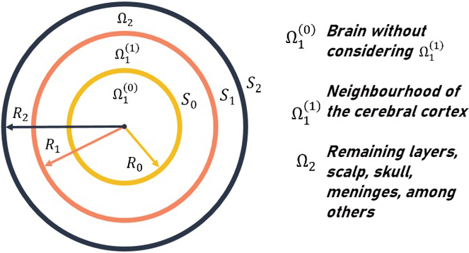
Source: Own elaboration.
Fig. 3 Schematic figure of volume conductor model, where
It will be convenient to denote
We consider the class
Where the corresponding series of Fourier coefficients
should converge.
Next, we solve the auxiliary contour problem ( 8 ), which in view of ( 17 ) means
compute A( f ). Since operator
A is linear and continuous, it is enough to compute
it is necessary to solve the associated contour problem
whose solution is imposed to take the form
It is easy to see that a (r) satisfies the equation
If we denote by
we arrive to functions
and the contour conditions at
Also, the following additional conditions must be added:
Solving this problem for
Thus, we finally get
In a similar fashion one obtains
Equipped with ( 84 ) and ( 85 ), we can easily write the resulting formula for A ( f ):
Finally, we must equate (86) and ( 45 ) and apply the coefficients unicity in order to obtain
Let us define
It is easy to see that
Let us write ( 87 ) in the form
or equivalently
This yields
Finally, have the sum for any positive integer n and
m from −n to n. If we
take into account that f is harmonic in
Consider the series with general term the second term of the left side of ( 96 ), which is equivalent to
Then the series with general term the right side of ( 96 ) also converges, whose terms are equivalent to
In this way, we arrive to the equivalent condition:
which turns to be the necessary and sufficient condition previously obtained for
V to be reproducible by an harmonic source defined in
Next, we will characterize the admissible data set corresponding to harmonic
sources in a neighborhood of the cortex. By Theorem 2 we have that, if
for
On the other hand, we have
So
Thus, from ( 98 ), ( 99 ) and ( 101 ) we get
also, from ( 94 ) we get
Making the computations, from ( 102 ) and ( 103 ) we get that
However, these classes
Then, we get
Starting from this development, and computing their coefficients via the equation Af = g as before, we get
From now, this subclass of harmonic sources will be denoted by
Note that sources class (107) precisely matches the set of sources that equal
harmonic sources in
The following result summarizes these results.
Theorem 5. If
In addition, the class
This last statement could result a little bit confusing; let us clarify this
point. By making use of the unicity of extension of harmonic functions, one can
identify a harmonic source in
Conclusions
In this article, a methodology for solving the inverse bioelectric source estimation problem in the brain, starting from instantaneous electroencephalographic measurements on the whole scalp, is proposed. We make use of a volume conductor model, in which the head and the brain are represented by means of concentric spheres outlining conducting layers with different but constant conductivities.
The main product of this work is the proposal of a general methodology for solving
the inverse electroencephalographic source estimation problem. Given an arbitrary
sources class
The process is basically as follows. First of all, one obtains the harmonic source which reproduces approximately the measurement, via the Admissible Data Method. Later, the specific source in a given class which best approximates the measurement is determined by using additional information provided by the harmonic source. The representing functions sets generating series development solutions and the computational approach depend on the geometric head model.
All this methodology can be extended to the case of time-dependent measurements (EEG), and provides algorithms for directly identifying time-dependent sources which do not depend on previous time discretizations. For the sake of clarity, this is out of the scope of the current work.
Finally, we want to make emphasis on the importance of Theorem 5. As a consequence,
we find that any measurement V in S2
can be reproduced by a harmonic source concentrated as close as wanted to the cortex
S1 . Furthermore, although these sources extend in a
unique way to

