


 text new page (beta)
 English (pdf)
 Article in xml format
 Article references
 Send this article by e-mail
 Cited by SciELO
  Similars in
SciELO
Similars in
SciELO 
 Permalink
Introduction
Automated image segmentation to detect domain-specific objects and elements is a challenging task in the image processing field because of high noise levels, low contrast and non-regular object shapes. Most state of the art methods segment images applying techniques focused into find predefined forms close to the shape of the searched objects. For example, for vessels detection in angiographic images, some methods try to approximate retinal arteries as tubular structures that are rotated at different orientations on the process. Other methods use the eigenvalues of a second order derivative of a Gaussian function in order to compute a vesselness measure to classify the vessel-like structures (Frangi, 1998; Wang, 2012). Due of the second derivative, detection process is highly sensitive to noise into the image. Even though the previous techniques has proven achieve good results, they are not optimal for crop detection since it is difficult to approximate crop shapes as tubular structures or continuos curves. For that reason, K-Means has been used widely into the crop image segmentation field (Jaware, 2012, p. 190; Patil, 2016). However, there exists other technique to segment images based on a concept called mathematical morphology. That method was proposed by Eiho and Qian and is widely used since it is governed by the parameters of size and shape of a structuring element (SE) (Eiho 1997, 696). This method uses the top-hat operator to enhance certain structures. Actually, the technique is well-known and canonical structuring elements like disk or rhombus are widely used. Due to the use of top-hat operator, this method has proved achieve good results in coronary vessels detection (Bouraoui, 2008, p. 1059; Sun and Sang, 2008). Also, performance and effectiviness of the original technique can be improved by using stochastic strategies like Genetic Algorithms (GAs) or Estimation of Distribution Algorithms (EDAs) (Cruz, 2015, p. 297; Guerrero-Turrubiates 2017, p. 1; Hauschild, 2011, p. 111). The morphological top-hat operator achieves a suitable performance for enhancing specific-domain objects; however, the process to determine the size and shape of the SE involves a trial-and-error stage or a selection based on an expert knowledge. To overcome the a-priori knowledge about the form and shape of the structuring element, an evolutive morphological descriptor is used in order to obtain a highly accurate SE by introducing the Univariate Marginal Distribution Algorithm (UMDA) for its design and the obtained results are better than K-Means technique and the Top-Hat operator using canonical shapes like disc and rhombus.
Method
Image Dataset. To measure the SE performance of the proposed method the crop-weed dataset was used. It contains a set of 60 crop image files with their respective ground-truth images (Haugh 2015, 105).
K-Means. The K-Means algorithm is a widely known unsupervised classification algorithm. It was proposed in 1967 by MacQueen (MacQueen, 1967). This technique requires a-priori to know the k value since it represents the number of clusters or classes to be formed by the process. On the successive steps, the technique initializes randomly k points that will be moved by an iterative process in order to form the final clusters automatically as described in Algorithm 1.

Fig. 1 shows an example of the classes (clusters) found by K-Means algorithm.
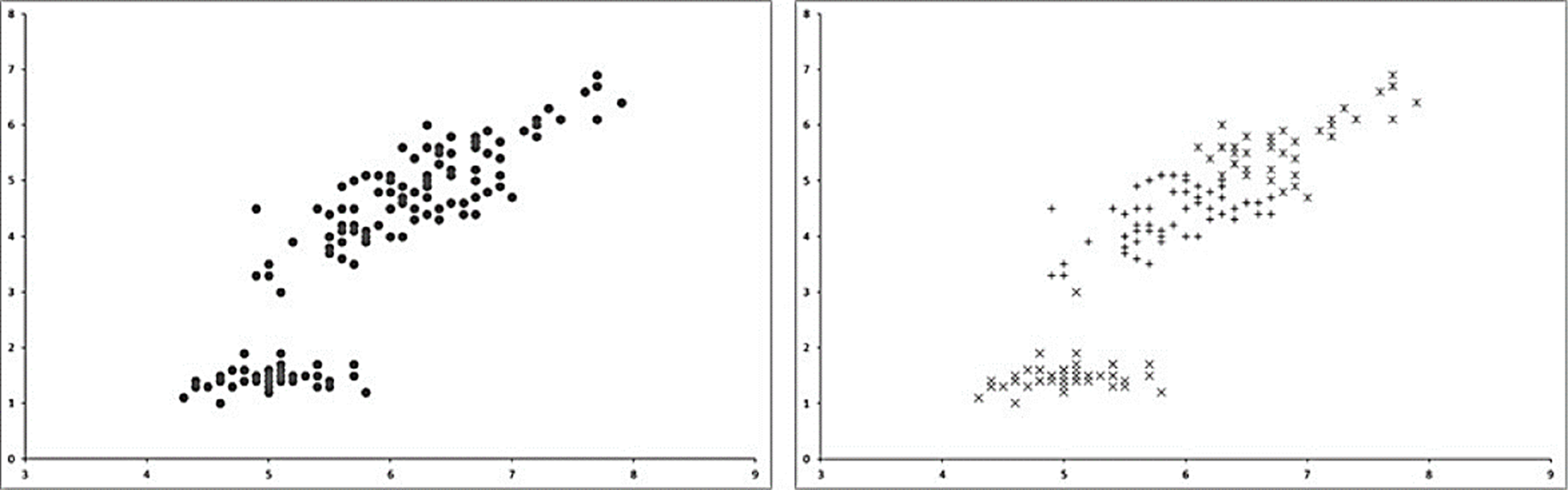
Fig. 1 Example of clusters formed by K-Means using k=3. On the left side the original dataset is represented. The right side shows the clustered data by the K-Means algorithm.
Main advantage of K-Means relies in the automatic classification made by an iterative process starting from several initial points called centroids wich are placed randomly across the data space and after moved or reallocated to their respective new clusters centers after each iteration. The process ends when centroids are not moved anymore. Although the algorithm is easy to implement, it could achieve to different classification results with the same data because of its stochastic centroids initialization.
Morphological top-hat operator. The morphological top-hat operator (Meyer, 1977) for grayscale images is part of the basic toolbox of mathematical morphology operators (Soille, 1999). Its function is to detect contrasted objects on non-uniform backgrounds. For grayscale images, there are two versions: the white top-hat which extracts bright structures and the black top-hat extracts dark structures. White top-hat operator is defined as the difference between an input image f and its opening as stated in Equation (1).
Where γ(f) denotes the opening operation.
On this research, the white top-hat was used since crops tends to be brighter than their surroundings and in addition, it corrects nonuniform lighting condition and make obvious contrast between background and objects. The performance of the top-hat operator depends on two factors: the shape and the size of the structuring element that is used. Fig. 2 shows a crop image with their corresponding ground-truth image outlined by a specialist on first column. Remaining columns shows the response of the top-hat operator using different shapes and sizes.
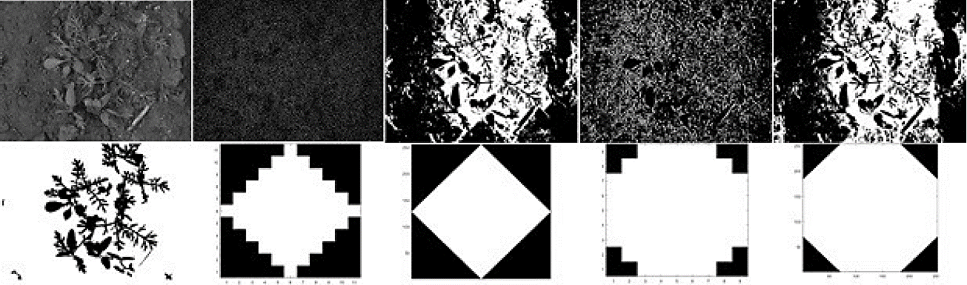
Fig. 2 First column: Original crop image on first row and their corresponding ground-truth on second row. Second column: On first row, the top-hat response; on second row the diamond shape (with size = 5) used as structuring element. Third column: On first row, the top-hat response; on second row, the diamond shape (with size=127) used as structuring element. Fourth column: On first row, the top-hat response; on second row, the disk shape (with size=5) used as structuring element. Fifth column: On first row, the top-hat response; on second row, the disk shape (with size=127) used as structuring element. For purposes of better visualization, contrast was improved on images placed in first row from columns 2 to 5.
Univariate Marginal Distribution Algoritm. UMDA is a population
technique-based like Genetic Algorithms (GA) (Heinz,
2001, p. 135). Instead of the population recombination and mutation
concepts, UMDA use the frequency of components in a population of candidate
solutions in the construction of new candidate solutions. Each individual in the
population is formed by a bit-string and it is denoted as:
xi =
[xi,1,
xi,2,…,.xi,D
] and each element xi,j
is called a gene. An array of vectors

Adaptive Morphological Descriptor. Based on the methods described above, a morphologic descriptor is generated in the form of a structuring element (SE) that is used with the top-hat operator in order to segment crop images. Main advantage of this approach relies in the construction of a SE based on the crop image features rather than a predefined or empirical shape. This method is focused in the generation of the best suitable SE by exploring the search space delimited by its size and finding the best pixels distribution along them. Also, the UMDA is used with a wide range of SE sizes to determine the best suitable morphologic descriptor avoiding an empirical trial and error procedure. Using this approach, the method can find and determine the shape and size of the SE in an automated way. In Fig. 3, six different SE’s generated by UMDA are presented.
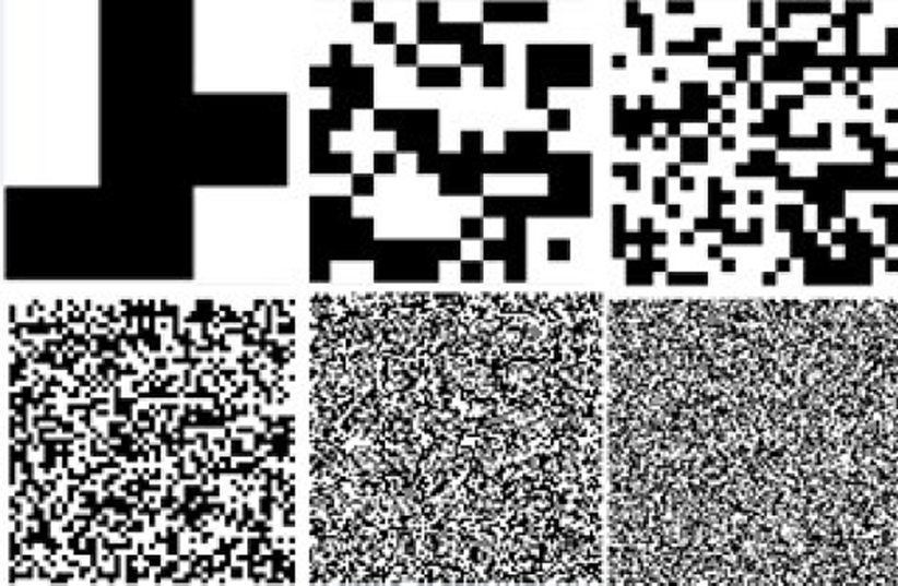
Fig. 3 Six different structuring elements generated by the UMDA. Sizes in pixels from left to right and up to down: 3x3, 13x13, 23x23, 49x49, 96x96 and 127x127.
Thresholding Otsu Method
Thresholding is an important technique in image segmentation applications. The basic idea of thresholding is to select an optimal gray-level threshold value for separating objects of interest in an image from the background based on their gray-level distribution. While humans can easily differentiable an object from complex background and image thresholding is a difficult task to separate them (Vala, 2013). Otsu method is type of global thresholding in which it depends only gray value of the image. Otsu method was proposed by Scholar Otsu in 1979. Otsu method is global thresholding selection method, which is widely used because it is simple and effective (Qu, 2010). The Otsu method requires computing a gray level histogram before running. However, because of the one-dimensional which only consider the gray-level information, it does not give better segmentation result. So, for that two-dimensional Otsu algorithms was proposed which works on both gray-level threshold of each pixel as well as its Spatial correlation information within the neighborhood. For that reason, Otsu algorithm can obtain satisfactory segmentation results when it is applied to the noisy images (Jian-zhuang 1991).
Once the image was segmented by using the top-hat operator a thresholding process is necessary in order to classify in a deterministic way those pixels belonging to conform crops from those that does not.
Evaluation Metrics
In order to asses the performance of the proposed method and select the best SE achieved by it, the receiver operating characteristic (ROC) curve graph and measures of sensitivity, specificity and accuracy were used (Zhu 2010). Also, the True-Positive Rate (FPR), True-Negative Rate (TNR), False-Positive Rate (FPR) and False-Negative Rate (FNR) metrics are used to measure the classifiers performance.
The TPR represents the fraction of elements that are positives and the classifier mark them as positives. The TNR represents the fraction of elements that are negatives and the classifier mark them as negatives. The FPR represent the fraction of elements that are negatives and the classifier mark them as positives. Fnially, the FNR represent the fraction of elements that are positives and the classifier mark them as negatives.
For this research the TPR represents the fraction of the crop pixels outlined by the specialist that are correctly detected by the method. The false-positive rate (FPR) is used to measure the proportion of actual negatives (non-crop pixels) that are incorrectly classified as positives (crop pixels). The TPR along the SE size provides information about how the SE shape and size is related with its performance to detect positive crops pixels.
By using TPR and FNR factors, the Sensitivity measure can be calculated by applying Eq. (2).
Eq. (3) is used to measure the the Specificity, which represents the non-crop pixels (background pixels) that are correctly detected as such by the method.
Accuracy represents the fraction of crop and non-crop pixels correctly detected by the method and is the most used measure to evaluate binary classification, which is defined in Eq.(4).
Where TPR and TNR represent the fractions of crop and non-crop pixels correctly segmented, and FPR and FNR the fractions of incorrectly classified pixels.
ROC graphs are another way besides confusion matrices to examine the performance of classifiers (Swets 1988, 1285). A ROC graph is a plot with the false positive rate on the x-axis and the true positive rate on the y-axis. The point (0,1) is the perfect classifier: it classifies all positive cases and negative cases correctly. It is (0,1) because the FPR is 0 (none), and the TPR is 1 (all). The point (0,0) represents a classifier that predicts all cases to be negative, while the point (1,1) corresponds to a classifier that predicts every case to be positive. Point (1,0) is the classifier that is incorrect for all classifications. In many cases, a classifier has a parameter that can be adjusted to increase TPR at the cost of an increased FPR or decrease FPR at the cost of a decrease in TPR. Each parameter setting provides a (FPR, TPR) pair and a series of such pairs can be used to plot a ROC curve. A non-parametric classifier is represented by a single ROC point, corresponding to its (FPR, TPR) pair.
Experiment
Since the top-hat operator is governed by the size and shape of the SE, a wide range of sizes were used on the performed tests starting with a 1x1 up to 127x127 pixels. In order to measure how the shape of an auto-generated SE influences the result, the UMDA was performed 30 times on each test image selecting the best achieved solution for each of them. The UMDA parameters were set as: 30 individuals, 30 generations and a selection rate of 0.70. The number of genes for each individual was set on 1, 9, 25, …, 16129, as each test was varying the SE size beginning with a size of 1x1 and finishing with a size of 127x127. These values were determined according to the best tradeoff between detection performance and computational time (Alba, 2006, p. 242; Cruz, 2015, p. 297; Hisashi, 2003, p. 112; Marler, 2010, p. 853; Topon, 2003, p. 1259). The final black and white image was obtained using the Otsu method. To assess the obtained results, the corresponding ground-truth for each test image was used. Ground-truth images are created from their corresponding originals and outlined by specialists. Since main goal of automated computing processing is trying to emulate human intelligence, the ground-truth elements provide an initial base to compare results obtained by automated computing algorithms. However, there does not exists a unique “truth” since two different human experts can achieve different results for the same problem or element. In the process of attempting to evaluate several recognition algorithms an uncovered number of serious hurdles with the ground-truthing elements are present. This problem may, in fact, be much more dificult than it appears. Ground-truthing is so hard, including the notions that there may exist more than one acceptable “truth” and/or incomplete or partial “truths” (Hu, 2001). Even though expert outlined ground-truth images could not represent a complete “truth”, they provide an initial base to measure automated computing results. This is the main reason why the ground-truth images provided by the dataset were used to assess the results.
The tests were performed over an Intel i7-4770 processor at 3.40 GZ with 8GB of RAM. All the tests were programmed on Matlab. The mentioned hardware and software was provided by the Universidad Tecnológica de León.
Results
After tests execution important results were obtained, and they are explained on this section. The performance results obtained for each image segmentation using the SE’s generated by UMDA are described in Table 1.
Table 1 Performance results obtained for each segmented image using the SE’s generated by UMDA.
| File | Accuracy | TPR | TNR | FPR | FNR |
|---|---|---|---|---|---|
| 001_Image.png | 0.9445 | 0.7590 | 0.9843 | 0.0157 | 0.2410 |
| 002_Image.png | 0.9424 | 0.7865 | 0.9624 | 0.0376 | 0.2135 |
| 003_Image.png | 0.9495 | 0.7992 | 0.9631 | 0.0369 | 0.2008 |
| 004_Image.png | 0.9518 | 0.8005 | 0.9712 | 0.0288 | 0.1995 |
| 005_Image.png | 0.8338 | 0.8728 | 0.8314 | 0.1686 | 0.1272 |
| 006_Image.png | 0.9632 | 0.7421 | 0.9879 | 0.0121 | 0.2579 |
| 007_Image.png | 0.9486 | 0.7708 | 0.9830 | 0.0170 | 0.2292 |
| 008_Image.png | 0.9446 | 0.7581 | 0.9644 | 0.0356 | 0.2419 |
| 009_Image.png | 0.9607 | 0.8120 | 0.9749 | 0.0251 | 0.1880 |
| 010_Image.png | 0.9509 | 0.8358 | 0.9593 | 0.0407 | 0.1642 |
| 011_Image.png | 0.9510 | 0.7853 | 0.9641 | 0.0359 | 0.2147 |
| 012_Image.png | 0.7952 | 0.9574 | 0.7899 | 0.2101 | 0.0426 |
| 013_Image.png | 0.9484 | 0.7597 | 0.9647 | 0.0353 | 0.2403 |
| 014_Image.png | 0.9515 | 0.8745 | 0.9550 | 0.0450 | 0.1255 |
| 015_Image.png | 0.8608 | 0.7804 | 0.8660 | 0.1340 | 0.2196 |
| 016_Image.png | 0.9472 | 0.7867 | 0.9625 | 0.0375 | 0.2133 |
| 017_Image.png | 0.9558 | 0.8029 | 0.9641 | 0.0359 | 0.1971 |
| 018_Image.png | 0.9553 | 0.7746 | 0.9711 | 0.0289 | 0.2254 |
| 019_Image.png | 0.8437 | 0.8903 | 0.8416 | 0.1584 | 0.1097 |
| 020_Image.png | 0.7456 | 0.9428 | 0.7421 | 0.2579 | 0.0572 |
| 021_Image.png | 0.8131 | 0.8900 | 0.8113 | 0.1887 | 0.1100 |
| 022_Image.png | 0.9447 | 0.8023 | 0.9536 | 0.0464 | 0.1977 |
| 023_Image.png | 0.9673 | 0.7874 | 0.9805 | 0.0195 | 0.2126 |
| 024_Image.png | 0.9686 | 0.8111 | 0.9784 | 0.0216 | 0.1889 |
| 025_Image.png | 0.9125 | 0.8505 | 0.9170 | 0.0830 | 0.1495 |
| 026_Image.png | 0.9499 | 0.6633 | 0.9648 | 0.0352 | 0.3367 |
| 027_Image.png | 0.9351 | 0.8163 | 0.9444 | 0.0556 | 0.1837 |
| 028_Image.png | 0.9519 | 0.7575 | 0.9760 | 0.0240 | 0.2425 |
| 029_Image.png | 0.9324 | 0.7422 | 0.9775 | 0.0225 | 0.2578 |
| 030_Image.png | 0.8057 | 0.9448 | 0.8025 | 0.1975 | 0.0552 |
| 031_Image.png | 0.9075 | 0.5584 | 0.9639 | 0.0361 | 0.4416 |
| 032_Image.png | 0.9464 | 0.7941 | 0.9630 | 0.0370 | 0.2059 |
| 033_Image.png | 0.9606 | 0.7840 | 0.9775 | 0.0225 | 0.2160 |
| 034_Image.png | 0.9540 | 0.7703 | 0.9761 | 0.0239 | 0.2297 |
| 035_Image.png | 0.9410 | 0.7553 | 0.9562 | 0.0438 | 0.2447 |
| 036_Image.png | 0.9470 | 0.7093 | 0.9808 | 0.0192 | 0.2907 |
| 037_Image.png | 0.8675 | 0.8861 | 0.8667 | 0.1333 | 0.1139 |
| 038_Image.png | 0.9340 | 0.7390 | 0.9620 | 0.0380 | 0.2610 |
| 039_Image.png | 0.8688 | 0.8489 | 0.8695 | 0.1305 | 0.1511 |
| 040_Image.png | 0.9141 | 0.6601 | 0.9487 | 0.0513 | 0.3399 |
| 041_Image.png | 0.9642 | 0.8056 | 0.9732 | 0.0268 | 0.1944 |
| 042_Image.png | 0.9627 | 0.8078 | 0.9698 | 0.0302 | 0.1922 |
| 043_Image.png | 0.8842 | 0.8911 | 0.8840 | 0.1160 | 0.1089 |
| 044_Image.png | 0.9731 | 0.7626 | 0.9797 | 0.0203 | 0.2374 |
| 045_Image.png | 0.9597 | 0.7823 | 0.9742 | 0.0258 | 0.2177 |
| 046_Image.png | 0.9792 | 0.8663 | 0.9820 | 0.0180 | 0.1337 |
| 047_Image.png | 0.9446 | 0.8329 | 0.9483 | 0.0517 | 0.1671 |
| 048_Image.png | 0.9340 | 0.8443 | 0.9378 | 0.0622 | 0.1557 |
| 049_Image.png | 0.9585 | 0.7636 | 0.9661 | 0.0339 | 0.2364 |
| 050_Image.png | 0.7643 | 0.9525 | 0.7612 | 0.2388 | 0.0475 |
| 051_Image.png | 0.9534 | 0.7643 | 0.9871 | 0.0129 | 0.2357 |
| 052_Image.png | 0.9475 | 0.8136 | 0.9648 | 0.0352 | 0.1864 |
| 053_Image.png | 0.9085 | 0.7174 | 0.9206 | 0.0794 | 0.2826 |
| 054_Image.png | 0.9637 | 0.8040 | 0.9830 | 0.0170 | 0.1960 |
| 055_Image.png | 0.9584 | 0.8197 | 0.9732 | 0.0268 | 0.1803 |
| 056_Image.png | 0.9464 | 0.7746 | 0.9691 | 0.0309 | 0.2254 |
| 057_Image.png | 0.9413 | 0.7808 | 0.9604 | 0.0396 | 0.2192 |
| 058_Image.png | 0.9443 | 0.7848 | 0.9718 | 0.0282 | 0.2152 |
| 059_Image.png | 0.9487 | 0.8020 | 0.9677 | 0.0323 | 0.1980 |
| 060_Image.png | 0.9648 | 0.7965 | 0.9857 | 0.0143 | 0.2035 |
In Table 2, is presented a summarized set of records containing the calculations of TPR and FPR that conforms the ROC for the two classic and the adaptive SE. Table rows were summarized to present the most significant SE sizes were the curve changes their behavior and takes their final stability.
Table 2 Summary of TPR and FPR calculations for the disk, diamond and autogenerated SE shapes. Summary was formed with the first 5 records containing SE size in a range from 1 to 9, second set of 5 rows contains SE size in a range from 65 to 73 and, last set of 5 rows contains SE size from 119 to 127.
| SE Size | Disc | Diamond | Adaptive | ||||||
|---|---|---|---|---|---|---|---|---|---|
| Accuracy | TPR | FPR | Accuracy | TPR | FPR | Accuracy | TPR | FPR | |
| 1 | 0.7625 | 0.1922 | 0.1875 | 0.7625 | 0.1922 | 0.1875 | 0.9198 | 0.0000 | 0.0000 |
| 3 | 0.8101 | 0.2393 | 0.1387 | 0.8191 | 0.2362 | 0.1283 | 0.8000 | 0.1570 | 0.1437 |
| 5 | 0.8663 | 0.2547 | 0.0782 | 0.8716 | 0.2641 | 0.0730 | 0.8308 | 0.2017 | 0.1135 |
| 7 | 0.8902 | 0.3481 | 0.0596 | 0.8875 | 0.3299 | 0.0611 | 0.8604 | 0.2324 | 0.0827 |
| 9 | 0.8991 | 0.4109 | 0.0554 | 0.8974 | 0.3934 | 0.0557 | 0.8799 | 0.2722 | 0.0647 |
| 65 | 0.9098 | 0.8319 | 0.0790 | 0.9145 | 0.8276 | 0.0737 | 0.9261 | 0.8005 | 0.0594 |
| 67 | 0.9079 | 0.8321 | 0.0810 | 0.9135 | 0.8286 | 0.0749 | 0.9253 | 0.8050 | 0.0607 |
| 69 | 0.9084 | 0.8328 | 0.0804 | 0.9121 | 0.8287 | 0.0763 | 0.9253 | 0.8068 | 0.0609 |
| 71 | 0.9077 | 0.8331 | 0.0813 | 0.9110 | 0.8295 | 0.0775 | 0.9240 | 0.8115 | 0.0625 |
| 73 | 0.9074 | 0.8342 | 0.0817 | 0.9111 | 0.8300 | 0.0774 | 0.9232 | 0.8133 | 0.0635 |
| 119 | 0.9033 | 0.8304 | 0.0853 | 0.9053 | 0.8322 | 0.0837 | 0.9116 | 0.8322 | 0.0771 |
| 121 | 0.9047 | 0.8294 | 0.0838 | 0.9046 | 0.8323 | 0.0843 | 0.9116 | 0.8335 | 0.0774 |
| 123 | 0.9035 | 0.8301 | 0.0851 | 0.9038 | 0.8322 | 0.0850 | 0.9108 | 0.8347 | 0.0783 |
| 125 | 0.9043 | 0.8302 | 0.0843 | 0.9029 | 0.8315 | 0.0860 | 0.9105 | 0.8340 | 0.0785 |
| 127 | 0.9040 | 0.8297 | 0.0846 | 0.9028 | 0.8314 | 0.0860 | 0.9101 | 0.8345 | 0.0790 |
Fig. 4 shows the performance averages for the accuracy and the SE size in a range from 1 to 127.

In Fig. 5 the performance for each shape is presented separately.
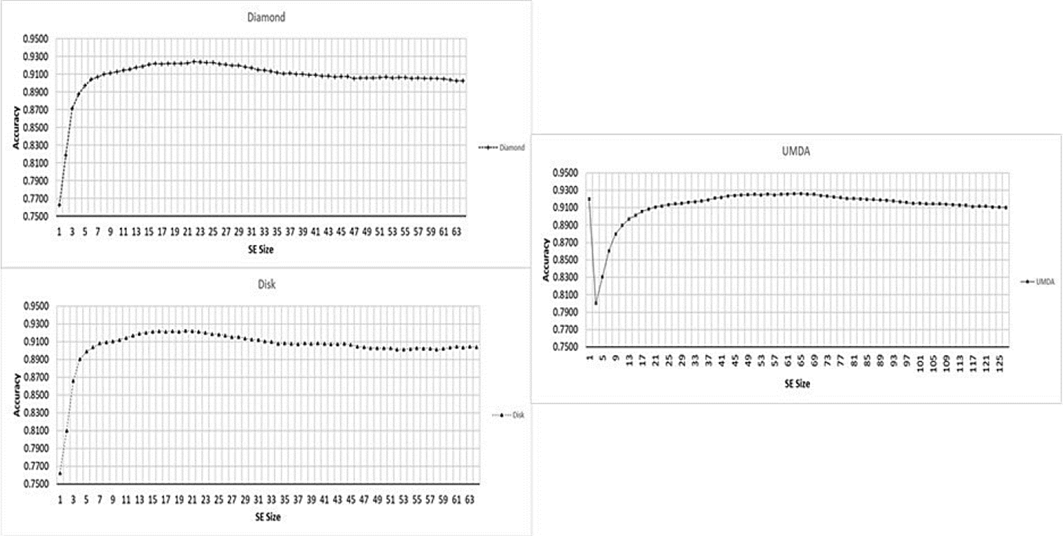
Fig. 5 Performance for different SE sizes, from 1x1 to 127x127 (x-axis) and Accuracy mean (y-axis) for each shape type.
In Fig. 6 the ROC curve is shown in order to know the best structuring SE size by contrasting TPR and FPR factors for different types of SE’s. The studied parameter to measure the classifier performance was the SE size.
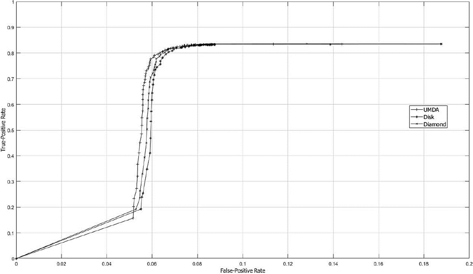
Fig. 6 ROC curves graph using SE sizes from 1x1 to 127x127. The SE size was the varying parameter used to study the classificatory performance. The FPR and TPR are represented on the x-axis and y-axis, respectively.
By contrasting Accuracy and ROC performances, the best result was obtained with a SE of 65x65 pixels. Fig. 7 shows a sample of the best SE’s achieved by UMDA.

In Fig. 8 the Accuracy comparison between the K-Means algorithm and the top-hat operator with their SE variants is shown.
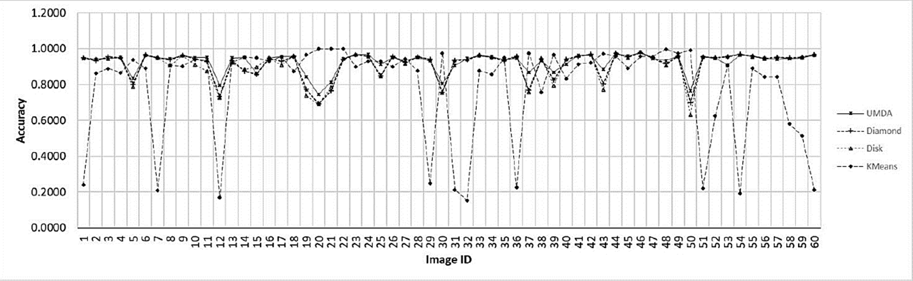
Fig. 8 Accuracy chart for the evaluated methods for each image. The x-axis contains each image ID. The y-axis contains the best achieved accuracy value by each method.
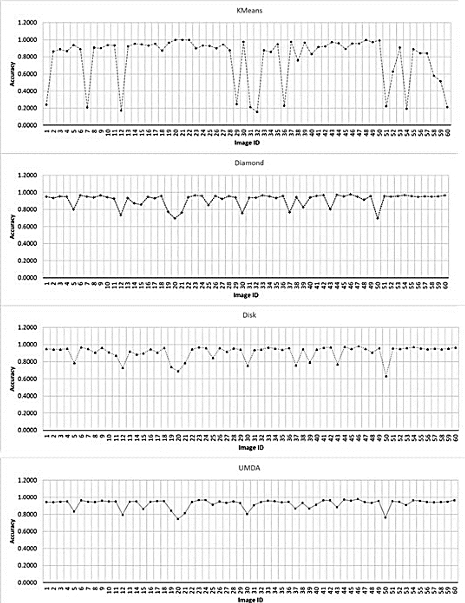
The Fig. 9 presents the accuracy results separated by each method.
Discussion
After test execution, the best performance was achieved by the top-hat operator using the UMDA generated structuring elements and it was verified contrasting the ROC curve graph with the performance data. Figs. 10 and 11 shows a subset of 5 images with their respective ground-truth and responses by the various methods applied for its segmentation.

Fig. 10 Subset of segmented images applying the K-Means method and the top-hat operator. From left to right, first column shows the original crop image; second column shows the ground-truth image; third column shows the K-Means segmentation result; fourth column shows the top-hat operator response using a disk SE with size of 65x65; fifth column shows the top-hat operator response using a diamond SE with size of 65x65; last column shows the top-hat operator response using the adaptive SE generated by UMDA with size of 65x65.

Fig. 11 Subset of segmented images applying the K-Means method and the top-hat operator. From left to right, first column shows the original crop image; second column shows the ground-truth image; third column shows the K-Means segmentation result; fourth column shows the top-hat operator response using a disk SE with size of 65x65; fifth column shows the top-hat operator response using a diamond SE with size of 65x65; last column shows the top-hat operator response using the adaptive SE generated by UMDA with size of 65x65.
The segmentation results achieved by K-Means shows difficulties to segment crop images with low contrast obtaining high rates of false-positives in most of them. The top-hat operator with disk and diamond shapes perform better than K-Means algorithm however, most of crops has an uneven shape and size including a low contrast with the background. For that reason, the adaptive shape improves all performance factors under a certain SE size as presented in Fig. 5. Since white top-hat operator removes objects with less size than the structuring element, the UMDA was able to evaluate multiple combinations of shapes and sizes, selecting the best overall size for the structuring elements. Also, the structuring elements builded by UMDA performs better removing non-crop pixels than classic shapes as it was illustrated in Figs. 10 and 11 in the last column. As presented in Fig. 12, the adaptive SE achieved a better result than rest of techniques because it was able to remove more non-crop pixels in the original image.
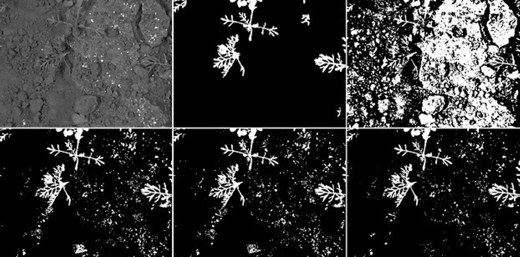
Fig. 12 Example of a crop image with low contrast and its segmentation results. From left to right and up to down: the original crop image; the ground-truth delined by an specialist; the result achieved by K-Means; the result achieved using the top-hat operator with 65x65 disk SE; the result using the top-hat operator with 65x65 diamond SE; the result using the top-hat operator using a 65x65 adaptive SE.
According with ROC curve graph presented in Fig. 5, the adaptive SE appears to achieve better results and, considering the original image resolution that is 1296x966 pixels, the differences with other methods become more significant. Also, the the accuracy performance was contrasted with the ROC curve since considering only the accuracy measure can conduct to wrong results and missinterpretations as described by (Zhu, 2010). For example, one of the highest accuracy performances was achieved using an adaptive SE with size of 1x1. However, making a closer view in data presented at Table 2 and contrasting with ROC curve presented in Fig. 6, the true-positive fraction was very low compared with a SE with size of 65x65 were the true-positive fraction assesses the accuracy factor.
Also, it is important to realize about the SE shapes and their content. For example, disk and diamond SE’s are solid shapes unlike those generated by UMDA since it has not restrictions in any way. This means for example, that disk and diamond shapes has not empty regions inside unlike those achieved by UMDA. Due to the presence of empty regions inside of the adaptive SE’s the removal or keeping of certain elements inside the image could be done in a wrong way by the processes of erosion and dilation performed by the top-hat operator. This is an important issue to be addressed and studied on future research works since it could conduct to improve the results by adding shape restrictions to the UMDA. Based on this study, future work will be related to reduce the decay rates by adding constraints to the search strategy in order to overcome current issues and also, as a mean to generate a robust set of structuring elements that could be applied to a wide variety of sizes and sizes of crops into digital images.

