


 nueva página del texto (beta)
 Inglés (pdf)
 Artículo en XML
 Referencias del artículo
 Enviar artículo por email
 Citado por SciELO
  Similares en
SciELO
Similares en
SciELO 
 Permalink
Introduction
Digital retinal images are used in the diagnosis of some ophthalmic pathologies, such as diabetic retinopathy. Common approaches to identify retinal pathological conditions rely on comprehensive dilated eye exams such as visual acuity, tonometry (internal eye pressure), pupil dilation, and optical coherence tomography (Fong et al., 2004; Lee, Wong, & Sabanayagam, 2015). In these approaches, the physicians search for a number of indicators including progressive changes in the retinal vasculature, leaking vessels, signs for potential vessel leakage (fat deposits), pupil structural integrity, damage of the nerve tissue, among others. Unfortunately, all these indicators manifest clearly only until advanced stages. It is the identification of minute changes in the retinal vasculature which can allow for reliable diagnosis at early stages. Thus, suitable computer-aided diagnosis tools are needed for the automated image detection of retinal pathology, and in general for the segmentation of the vascular tree, as it is an important indicator not only of diabetes-related conditions but also for the diagnosis, screening, treatment, and evaluation of various cardiovascular, neurovascular, and ophthalmologic diseases such as hypertension, arteriosclerosis, and choroidal neovascularization (Abràmoff et al., 2010; Muangnak et al., 2015; O’Hara, 2004).
According to the World Health Organization, diabetes is at epidemic levels worldwide, and developing countries face the greatest risk (King & Rewers, 1993; Popkin et al., 2012). In those countries, a number of public health issues are rooted in the high levels of obesity that are now one of their typical characteristics. For instance, in Mexico, diabetes is at pandemic levels, data from 2016 suggested that the prevalence of diagnosed diabetes increased from 7.6% to 9.4% in ten years (Arredondo, 2018; Instituto Nacional de Salud Pública, 2016). A common consequence of chronically high blood sugar levels from diabetes is the damage of the retinal vasculature, which leads to diabetic retinopathy, and eventually to blindness (Fong et al., 2004). In this regard, diabetic retinopathy is the most frequent cause of vision loss worldwide (Lee et al., 2015) and, in the particular case of developing countries, it is the first cause of blindness in working-age adults (Cervantes-Castañeda et al., 2010).
The assessment of anomalies in retinal vessels used to be a time-consuming task since high skilled technicians were required to assess the images and the diagnostic was based on their experience (Niemeijer et al., 2004). This methodology presented serious drawbacks due to i) the scarce availability of such skilled technicians, and ii) the diagnostic was prone to appreciation errors. For these reasons, there has been an increasing interest in the development of automatic of assessment techniques (Fathi & Naghsh-Nilchi, 2013; Kuri, 2015; Siddalingaswamy & Prabhu, 2010). These new tools do not intend to deprecate medical diagnosis but to contribute to it. At the same time, these implementations have to be efficient regarding computation time and data management to reduce the human workload, to overcome the bottlenecking problems associated with screening programs, and to enable high-throughput workflows (Jelinek & Cree, 2009). Moreover, those automatic tools are desired to operate based on self-contained metrics, in order to eliminate human biases. However, one of the biggest challenges is the determination of the accuracy in the vessels detection in the presence of discontinuities in the vascular structures (Gegundez-Arias et al., 2012; Yan et al., 2018).
In this study, a method for comparison of segmented retinal blood vessel images is presented. The method is used to compare the vessel segmentation obtained by a simple automatic segmentation against manually segmented images. Our approach is based on linking the standard performance metrics, which are calculated blindly from the outcomes of a generic segmentation algorithm, with the actual structural properties of the images by using the fractal dimension (FD). Unlike other studies, here we do not attempt to give a diagnosis relying on the value of the FD, but to use it as an auxiliary figure of merit to optimize the performance of the segmentation algorithm. The methodology presented i.e., correlations between structure and segmentation metrics, is general and it does not depend on the particular segmentation algorithm used. Standard linear regression analysis shows that some of the standard metrics strongly depend on the image complexity regardless of the sub-regions in which the original image is divided. Our results show that the FD of the bit-wise difference between two images contains information statistically insightful on the algorithm’s capability to segment the vasculature.
Method
A plethora of techniques, algorithms, and methodologies for the segmentation of retinal blood vessels can be found in the literature (Abràmoff et al., 2010; Fathi & Naghsh-Nilchi, 2013; Felkel et al., 2001; Garg & Gupta, 2016; Jelinek & Cree, 2009; Kolar et al., 2013; Kuri, 2015; Siddalingaswamy & Prabhu, 2010). A particularly useful reference for the present work is Ref. (Vostatek et al., 2017) as it includes algorithms (both supervised and unsupervised) with publicly available implementations. Often in solving a segmentation problem, multiple techniques are used together. Thus, a unique classification of the different algorithms is not feasible. Based on the image processing methodology employed, the techniques used for the segmentation of the retinal vascularity can be classified in a more or less consistent manner as supervised and unsupervised classification methods, matched filtering approaches, morphological operations, and deformable models (Garg & Gupta, 2016). Other more specific categorizations propose vessel tracking, multi-scale approaches, and vessel profiling as independent classifications from the more general morphology-based techniques (Fraz et al., 2012; Kirbas, C. Quek, 2004), and intensity-based segmentation algorithm (Gonzalez & Woods, 2001). However, we would like to emphasize that our approach is not exclusive to a particular algorithm and the same methodology i.e., correlation analysis between standard performance metric and FDs, can be used irrespectively of the segmentation algorithm of choice.
The retinal images are from the DRIVE database (Niemeijer et al., 2004), which contains TIFF color images of 565 × 584 pixels. For each original, colored image, this database provides two manually labeled masks (binary images) where the retinal vasculature is indicated. Ideally, these two reference masks should be equal, however, as it will be shown later, they are not. The first step is to split the red, green, and blue channels of the original image. Fig. 1 shows the original image and the grayscale images of the red, green, and blue channels, respectively. In our case, only the green channel was used since it provides the best contrast with respect to the others.
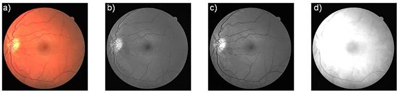
Fig. 1 The original image (a), grayscale images of the (b) blue, (c) green, and (d) red channels respectively
Despite inherently providing the best contrast, the green channel can be improved, since in some regions information can be lost due to over-brightness (see Fig. 2). To solve this problem, the CLAHE adaptive histogram equalization is used (Pizer et al., 1987; Zuiderveld, 1994). The image is divided into 17×17 sub-images, and then each of these blocks is histogram equalized, with a contrast limit of 2. In other words, if any histogram bin is above the specified contrast limit, those pixels are clipped and distributed uniformly to other bins before the histogram equalization. After equalization, a bilinear interpolation is applied in order to remove artifacts in the tile borders. Then, a Gaussian blurring is performed over the image (see Fig. 2(c)).
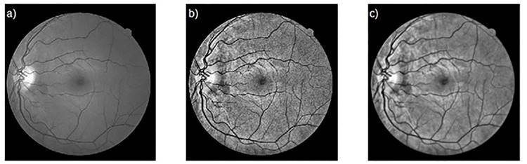
Fig. 2 Comparison between: (a) the green channel, (b) adaptive histogram equalized green channel, (c) Gaussian blurred image
The main goal of this process is to reduce the effects of high-contrast pixelation, which can be clearly noticed in Fig. 2(b). The Gaussian filter is applied using a mirror of 9 × 9 pixels, and the corresponding standard deviation of 2. The resulting image is further enhanced by applying a Laplacian operator and then performing a bit-wise subtraction to the blurred image. The last step is a Gaussian adaptive thresholding operation using a block size of 27 pixels. At this stage, morphological operations like erosion and dilation can be applied to improve the image in the case of pixelation. A summary of the algorithm is shown in Fig. 3.

Fig. 3 Schematic overview of the segmentation method used for these tests. The method comprises of green channel extraction, histogram equalization, Gaussian blurring, image enhancing and thresholding
Next, we describe our method for the comparison of segmented retinal blood vessel images that is based on linking the standard performance metrics with the structural properties of the images through the FD. Our approach can be readily extended to a more complete assessment by including metrics of the connectivity, area, and length of the segmented vessels (Aquino, Gegúndez, Bravo, & Marín, 2010; Garg & Gupta, 2016; Kolar et al., 2013).
Fig. 4 shows an example, from one of the images processed, of the original retinal picture, the automatically obtained image (generic algorithm; described in the next section), and the manually labeled images. It should be clear that despite the binary images look similar; they are not the same.

Fig. 4 Comparison of the different vascular images, (a) original image, (b) automatically extracted, (c) manually-labeled mask 1, (d) and manually-labeled mask 2
For our numerical experiments, we made use of the retinal images from the DRIVE database (Staal et al., 2004). Quantitative evaluation of the algorithm’s performance and the accuracy of the extraction of the vascular tree was done based on the difference between images resulting from the bit-wise (pixel-based) subtraction with the manual mask 2 as a reference, i.e. the difference between the binary images in Fig. 4.
Fig. 5 shows the difference images obtained between the automatically extracted image and the manually labeled 2 (between panels (b) and (d) in Fig. 4), as well as between the manually labeled images (between panels (c) and (d) in Fig. 4). There are important aspects that need to be highlighted. One can clearly see that there can be significant differences between the manually labeled images. These differences occur mainly in the small vessels, which are inherently difficult to identify and extract. More importantly, it can be seen that the small vessels in the difference image actually preserve their structure which means that even the manually labeled images can miss entire vascular ramifications. Realizing the existence of these differences between manually labeled images is of critical importance as they are used as the reference in automated processing. Conversely, when we compare the outcome of generic algorithm with the manually-labeled mask 2 (Fig. 5(a)), there is certainly an error, but there are not well defined vascular structures, and the white pixels are more uniformly distributed over the image. Thus, the algorithm can recover vascular structures, including thin vessels, with a small error, i.e. only short portions of the ramifications go undetected.
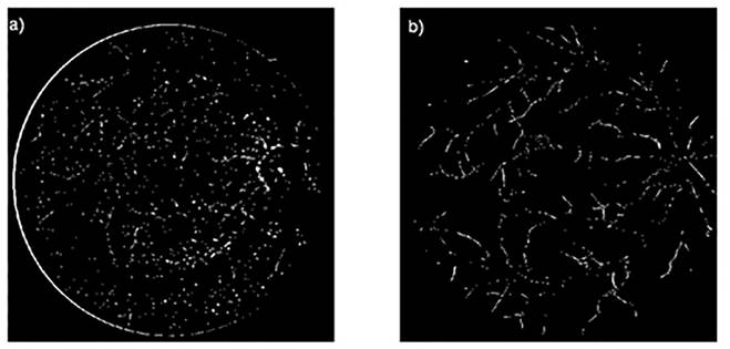
Fig 5. The bit-wise difference (pixel based subtraction) between the automatically extracted (a) and manually-labeled mask 2, and between the two manually labeled masks (b)
Both the segmentation algorithm and the evaluation algorithm were programmed in Python using OpenCV libraries, and the retina images and manual segmentations are taken from the DRIVE database.
Results
Standard metrics are commonly used to quantify the performance of the classifiers implemented for the extraction of retinal blood vessels from the fundus image. Given the nature of pixel-based classification i.e., whether the pixel belongs to a vessel or the surrounding tissue, four possible events can take place including correct and incorrect classifications. These are the so-called true positive (TP), true negative (TN), false positive (FP), and false negative (FN). TP and TN correspond to the correct classification of a pixel as part of a vessel or background, respectively, while FP and FN refer to the pixel’s misclassification. These four classification labels can then be used to construct the following performance metrics:
TPR (True Positive Ratio) is the ratio of pixels correctly detected as vessel pixels to the number of pixels present in vessel area i.e.
TNR (True Negative Ratio) is the ratio of number of pixels correctly identified as non-vessel pixel to the number of pixels present in the non-vessel area i.e.
FPR (False Positive Ratio) is the ratio of pixels erroneously identified as vessel pixels to the number of pixels present in the non-vessel area i.e.
FNR (False Negative Ratio) is the ratio of pixels erroneously identified as non-vessel pixels to the number of pixels present in the vessel area i.e.
Accuracy (ACC) is the ratio of total number of true events (TP+TN) to the total population (total number of pixels in the image) i.e.
Sensitivity (SN), which a different name for TPR, is a measure of the ability of the segmentation process to detect the vessel pixels and is defined as
Specificity (SP), which a different name for TNR, is a measure of the ability of the segmentation algorithm to detect background or non-vessel pixels and is defined as
The area under the Receiver Operating Characteristic (ROC) curve, or Area Under Curve (AUC), which is the plot of (1-SP) versus SN. The performance of the system is better if the curve approaches closer to the top left corner and equals 1 for optimal systems.
These metrics quantify the precision in the correct classification of the segmented pixels as part of the vessels or the background. Detailed comparisons between the performances of various retinal segmentation techniques, performing on databases available in the literature, especially DRIVE and STARE which are currently the most common datasets for the evaluation of retinal vessel segmentation methods, can be found in Refs. (Fraz et al., 2012; Garg & Gupta, 2016; Vostatek et al., 2017).
In Fig. 6 we summarize the standard performance metrics for the case where the automatically extracted mask is compared to the manually labeled mask 2, and for the case where the two manually labeled masks are compared to each other. The average value and the standard deviation are calculated from the 20 images tested. Both the table corresponding to the values shown in Fig. 6 (Table 1) and an extended table showing all the values obtained can be found in Tables 3-6 in the Appendix, at the end of this document.

Fig. 6 Graphical representation of the average value and the standard deviation for the standard metrics
From Fig. 6 it can be seen that the accuracy of generic algorithm is slightly lower than that from the manually labeled masks but, more importantly, the accuracy of manually labeled images does not reach 100% due to differences in the manual labeling. In any case, see Table 1 in the Appendix, it is the relative 2.3% error with respect to what can be manually labeled what can be taken as the accuracy of our approach.
Up to here, we have presented the results obtained by using standard metrics alone. In doing so, we noticed that vessels annotated by different observers may vary both in thickness and in location thus resulting in manually-labelled images that can be significantly different, as seen in Fig. 5 and Fig 6. These limitations impose the need for automatic, self-contained metrics that can reduces, or even eliminate, the human biases possibly involved.
In the following, we use the FD as an auxiliary self-contained metric that can help to connect the standard metrics of the algorithm, which are calculated blindly from the outcomes of the segmentation algorithm, to the actual structural properties of the image. It is well known that fractal geometry is an effective tool for the characterization of irregular shapes and that the FD can be a good descriptor of their complexity. In our case, since we are working with two-dimensional objects, i.e. planar images, the FD can lay between 1 and 2.
Some properties of fractals have been used in medical image analysis, for example for texture analysis (Chen, Daponte, & Fox, 1989; Lopes & Betrouni, 2009). In the case of the analysis of human retinal vessels, it has been reported that a healthy eye has an FD of around 1.7 (Family, Masters, & Platt, 1989; Mainster, 1990; Popovic et al., 2018). However, it has also been shown that, due to its underlying dependence on the structural properties of the image, the FD is sensitive to a number of other factors from both biological origin e.g., age, cataracts, and lens opacity (Cheung et al., 2012), changes in blood pressure due different origins (Sng et al., 2010; Zhu et al., 2014), existing diabetic condition (Aliahmad et al., 2014), and cognitive dysfunctions (Taylor et al., 2015), as well as numerical origin e.g., size and location of the region of interest (Aliahmad et al, 2014; Huang et al., 2015) or the specific stages in the pre-processing procedure (Che Azemin et al., 2016). Due to this overall ‘instability’ of the FD, which can be significant in some cases, one should not rely a quantitative analysis for diagnosis purposes solely on the value of the FD (Huang et al., 2015). In our approach, we do not attempt to provide a diagnosis using the FD, but to suggest its use as a feedback to the segmentation algorithm through its correlation with the standard metrics (see Fig 7).

Fig. 7 Flow diagram of the proposed fractal dimension-based correlation analysis. The upper dashed rectangle indicates the image segmentation (generic, intensity based algorithm in our case) while the bottom one indicates the proposed correlation-based analysis. Potentially, the outcome of this analysis can be used to calibrate the parameters involved in the segmentation to optimize the algorithm’s performance, as indicated by the dotted arrows
Following the so-called box counting method which is a common approach for this estimation, the FD can be approximated by the number of boxes needed to cover the object (N), and it typically increases slowly as we decrease the box size (r), then the FD is given by
In Fig. 8, the FD is presented as a function of the number of subdivisions for the raw binary masks (Fig. 8(a)) and for the difference images (Fig. 8(b)). The values plotted correspond to the average obtained from the 20 images processed; the error bar represents the standard deviation. From Fig. 8(a), the FD obtained from our approach closely matches that from the manually labeled mask 2. In terms of the difference images (Fig. 8(b)), the subtraction of the manually labeled masks leads to a smaller FD due to the presence of more organized structures i.e., conversely, the subtraction of the automatically extracted mask from the manually labeled one has larger FD due to the random pattern that covers the image more uniformly. The complete data set from which these values were extracted can be found in the Appendix.

Fig. 8 Fractal dimension, as a function of the number of sub-images: of the raw binary masks (a), and of the difference images obtained from the bit-wise (pixel-based) subtraction (b)
To quantitatively evaluate the relation between the FD and the standard metrics, a linear regression analysis was performed, and the Pearson’s correlation coefficient was calculated for the different data sets, e.g., the correlation between TNR and the FD using a different number of sub-images. Fig. 9 summarizes the correlation between all these datasets, the corresponding numerical values can be found in Table 2 in the Appendix. The algorithm is mildly sensitive to the identification of vessel pixels with respect to structure complexity, as indicated by the relatively low correlation between TPR and the FD, but its specificity i.e. identification of background, non-vessel pixels, strongly depends on the complexity of the structure. In other words, this means that the identification of vessel pixels is not critically compromised if the structure’s complexity increases, but the correct identification of background pixels will be more effective for simple structures.

Fig. 9 Pearson’s correlation between the standard metrics and fractal dimension as a function of the number of subimages analyzed
To exemplify one of the correlations in Fig. 9, the linear regression analysis is shown in Fig. 10(a) for the case where the FD is correlated with the TNR, for a different number of sub-images, as indicated. Fig. 10(b) shows the slope calculated from the linear regression analysis as a function of the number of sub-images. In this example, this plot indicates that the correlation between the FD and the TNR becomes stronger with increasing number of sub-images, but it also shows that this correlation saturates after a certain amount of sub-divisions.
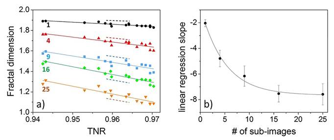
Fig. 10 a) Scatter plot showing the strong correlation, obtained from linear regression, between the fractal dimension of the difference images (automatic - manual 2) and the TNR standard metric. The strong correlation remains regardless of the number of sub-images. b) Dependence of the linear regression slope on the number of sub-images. The error bars indicate the standard error of the linear regression
Discussion
A method for comparison of segmented retinal blood vessel images based on the FD was presented. As an example, the method was used to compare the vessel segmentation obtained by automatic segmentation against manually segmented images. Linear regression analysis, on the standard metrics and image subdivision, showed that standard metrics strongly depend on the image complexity regardless of the sub-regions in which the original image is divided. As a consequence, small relative errors are found when using only standard metrics as a comparison. The use of the FD as an auxiliary, self-contained metric, together with subdividing the images under study, help us to further identify the nature of the differences between segmentations methods. Thanks to the fact that the strong correlation between the standard metrics and the FD is preserved regardless of the size of the sub-images, the FD can be used as an automatic, self-contained feedback in an iterative segmentation algorithm, for instance, to optimize the size of the region of interest in order to minimize the dependence of the algorithm’s performance on the actual properties of the image, that can be roughly summarized as
Finally, we highlight that our approach is compatible, and can be used in a complementary manner, with similarity assessment approaches which are based on other aspects the image’s structure such as connectivity, area, and the length of the segmented vessels (Vostatek et al., 2017), or the so-called skeleton maps (Fraz et al., 2012; Kirbas, C. Quek, 2004). This may lead to the development of calibration and optimization approaches that are based on a set of automatic, self-contained geometrical descriptors simultaneously, all of which are related to different aspects of the images structure. In clinical applications, such an approach could greatly improve the quality and accuracy of the outcome of a segmentation stage.

