


 nueva página del texto (beta)
 Inglés (pdf)
 Artículo en XML
 Referencias del artículo
 Enviar artículo por email
 Citado por SciELO
  Similares en
SciELO
Similares en
SciELO 
 Permalink
Introduction
There are areas in Mexico that are neither rural nor urban. Supposedly these areas are: 1) economically heterogeneous, and 2) economically different from those considered as rural and from those considered as urban. The motivation for this work was to formally prove whether these statements are true by using statistical analysis that consider that data come from geographical information. For statement 1) we compare populations by using and comparing different models that consider different assumptions, some of which are closer to create a model that accommodates to the geographical information features. To answer statement 2), we also compare populations, but we observe that a model considering the geographical dependence of the variable analyzed should be preferred.
It is well known that a one-factor ANOVA, as described e.g. in (Kutner et al., 2005) or (Montgomery, 2009, ch. 3), can be used to compare three or more populations through their associated means. There are some assumptions this model requires inherited from its corresponding associated linear model so that it can be used only for specific types of data. When such assumptions are not satisfied, an equivalent non-parametric test, the Kruskal-Wallis test, can be used. There are data in which observations belong to the same individual, for instance when we have a spatial unit and there is a variable that can be measured k times. This can be thought of as having an individual providing information for the different populations we want to compare. In this case the independence between observations, understanding them as the combination between individual and one of the k measures, assumed for the corresponding one-factor ANOVA is not satisfied and it is necessary to use an alternative model, a repeated measures model. According to the data, it could even be sensible to use an equivalent non-parametric test, the Friedman test.
One assumption in a one-factor ANOVA corresponds to independence between the observations; however, it could be violated specially for data involving time or spatial information. In the last case, this information can be included in the linear model. There are different models of this kind; we use here a geographically weighted regression (GWR), which was introduced in (Brunsdon et al., 1996), (Brunsdon et al.,1998), and (Fotheringham et al., 1998), modified to include global and local parameters in (Brunsdon et al., 1999), and further discussed in (Fotheringham et al., 2002).
The models and tests are illustrated through two data sets. The first study corresponds to measurements of economical activity in different sectors in regions in Mexico that are neither rural nor urban. We compare the results obtained using each method by defining comparable measurement units and see how the different models are an improvement on creating a model whose assumptions are closer to the data structure. Supposedly all sectors should be equally important in these regions, but we formally show that in Mexico it is not the case and determine which are the most important sectors, which as far as we know has not been made before. The second study illustrates the GWR method using data concerning income in Mexico. We show how the independence between observations assumption is violated because there is spatial autocorrelation for both the variable analyzed and errors associated with a one-factor ANOVA. This study presents spatial autocorrelation due to that income is expected to be similar in neighbor regions. Then, we show that by fitting a GWR this problem is solved. We infer that there is a difference in income between rural, urban, and the neither rural nor-urban regions; and that the highest income belongs to the urban region followed by the neither rural nor urban region and finally by the rural region. The comparison is obtained through a post hoc analysis, which as far as we know has not been applied in these kind of models before.
This paper is organized as follows. In Section 2 we describe the data that motivated this work. In Section 3 we introduce two models, one-factor ANOVA and repeated measures models, and two tests, Kruskal-Wallis and Friedman tests, which are useful to compare distributions in populations, and analyze their relationship. We also introduce there the GWR method and describe a model including spatial information equivalent to the one-factor ANOVA to compare means. In Section 4 we illustrate the models and tests through the two data sets introduced above. We also show through simulated data that using an inadequate test can lead to different results. Finally, in Section 5 we present a discussion.
Data
Economic sectors difference. There are regions in Mexico that are neither rural nor urban. From the information provided by the National Survey on Occupation and Employment 2010 (ENOE 2010) and the National Population and Housing Census 2010, both in Mexico, we obtained a sample of 970 spatial units (s.u), localities in which Mexico is divided. They correspond to those s.u. whose population size is greater or equal than 2,500 or less or equal than 100,000. From the same data, we calculated a measure of the importance of each of five economic sectors in each s.u. called the localization ratio. If the sectors are not equally important this ratio should be different between them. In Section 4.1 we assess through four different methods that this statement is true and determine whether an economic activity is more relevant than the others.
Income difference. The data presented in Section 4.2 correspond to a sample of 2,049 spatial units in Mexico obtained also from the ENOE 2010 in which we generated a factor corresponding to type of locality according to their population size: less than 2,500, greater than 100,000, and localities whose population size is between 2,500 and 100,000. We calculated the total income in each s.u. We wanted to know whether the distribution of income was the same between all three types of regions, and if differences were observed, in which type of locality there was the highest income.
Methods
Models and tests to compare populations and their relationship
Comparing populations methods assuming independent samples
Suppose there are k populations corresponding to independent random samples (there is independence between the elements in each sample and between samples) where the observation i in population j, j=1,…,k is denoted as O ij . Additionally, assume that they follow a normal distribution. A one-factor ANOVA is a linear model satisfying these assumptions which can be used to compare the means associated with those populations. It can be written as follows
where n j is the number of observations in population j, μ is a constant term, S corresponds to a variable that divides all observations into k populations, so that S j corresponds to a parameter for population j, and ε ij is a random error such that all errors are independent and ε ij ~ N(0,σ2), where σ2 is a positive constant term.
From the model, it can be inferred that O ij ~ N(μ,σ2), with μ j = μ + S j , so that testing if there is not effect of variable S on O ij , i.e. testing the null hypothesis H 0 : S 1 = S 2 = … = S k = 0, is equivalent to test that the means μ j are the same for all the k populations, assuming normality. As S is a factor, i.e. a categorical variable, used as an explanatory variable, identifiability conditions should be added to find one solution to the normal equations instead of a set of solutions. For instance, we create dummy variables for the first k - 1 populations or values of S. The linear model involving such dummy variables and the corresponding hypothesis tests are equivalent to the ones for S j . All the assumptions are equivalent to the ones used in a t-test to compare means between two independent samples, and that is why an ANOVA can be seen as its generalization. When the null hypothesis is rejected, it is possible to perform multiple comparisons. There are many of such comparisons, e.g. Tukey’s, Tamhane’s, Scheffe’s, Duncan’s, etc. Post hoc analysis were introduced in (Tukey, 1949), a review of them, for both the parametric and nonparametric case, can be found in (Day and Quinn, 1989), and a method based on ranks is developed for instance in (Dunn, 1964).
When data correspond to an ordinal scale or when normality is not satisfied, a test equivalent to the one given by the one-factor ANOVA corresponds to the Kruskal-Wallis test. All nonparametric tests mentioned in this paper are further discussed in (Conover, 1999). As many other non-parametric tests it is based on the ranks associated with the observations. In this case, the independence assumption still holds as in a one-factor ANOVA. The associated null hypothesis is H 0 All of the k distribution functions are identical, versus the alternative H 1: At least one of the populations tends to yield larger observations than at least one of the other populations. When the null hypothesis is rejected, it is possible to perform a post hoc analysis; there are several of such methods for comparing pairs of populations. One of them corresponds to apply Mann-Whitney U tests or Wilcoxon rank sum tests, which are equivalent to Kruskal-Wallis tests but considering only two independent populations, for each pair of groups, see e.g. (Kirk,1968, ch. 13), and after that to apply a Bonferroni correction to the significance obtained from the series of tests.
Comparing populations methods assuming related samples
When a variable S has k possible values, i.e. k possible populations can be derived from S, and when for each individual corresponding to a random sample we measure a variable in each value or category of S, we study related samples. If we want to compare the samples for the k populations, that is if we want to test whether the distribution of a variable in the categories in S is the same, then the independence assumption considered in the previous methods is not satisfied. In this case, a model analogous to the one-factor ANOVA corresponds to the repeated measures linear model as studied e.g. in (Kutner et al., 2005), (Vonesh and Chinchilli, 1997, ch. 3) where it is called a one-way repeated measures ANOVA, or in (Crowder and Hand, 1990, ch. 3).
One assumption that can be associated with a repeated measures model is sphericity, which means that the variances associated with the populations of differences is the same, as discussed in (Keselman et al., 2001). Sphericity also corresponds to having a variance and covariance matrix of type H. A hypothesis test concerning such structure is obtained through a likelihood ratio test known as Mauchly’s test, see (Vonesh and Chinchilli, 1997, p. 81, 85). Even though there is software that specifically fits such models, e.g. SPSS, they can also be fitted by using any software that fits linear models whenever sphericity is considered. To do this, we fit a two-factor ANOVA in which S and individual I are included as explanatory variables or factors. Consider that I i corresponds to the effect associated with individual i, then we have the model
where L is the number of individuals; μ, S and S j are the same as in model (1), and ε ij is a random error such that all errors are independent and ε ij ~ N (0,σ2), with σ2 a positive constant term.
Observe that in model (2) independence and homoscedasticidy of the errors are related to sphericity. This is because under such assumptions, for instance for populations 1 and 2,
We can fit the linear model (2) and determine if there is effect of variable S on O ij or we can directly fit the repeated measures model, for instance using SPSS, in which case the sphericity assumption is not necessary. In repeated measures models there are both between and within subjects effects, the former correspond to effects of variables measured once for each individual and the latter to effects of variables as S, which divides each individual into k observations. There are no between subjects effects and there is only one within subjects variable in the model considered here. The within subjects effects test can be used to determine if there is effect of variable S on O ij as in the ANOVAs analyzed before, its interpretation is the same. There are some specific tests where the results are adjusted when the sphericity assumption is not satisfied, e.g. the Greenhouse-Geiser univariate test, which corrects the degrees of freedom in the model assuming sphericity, see e.g. (Keselman et al., 2001), or Pillai’s multivariate test. All multivariate tests do not assume sphericity, they are based on multivariate analysis of variance (MANOVA) models as presented by (Cole and Grizzle, 1966). The multivariate tests used here are discussed for instance in (Crowder and Hand, 1990, p. 67-70).
When there is effect of S on O ij , i.e. the means are not he same between the k populations, we obtain multiple comparisons. This is equivalent to see if the estimated marginal means, i.e., the means under the model, corresponding to factor S are the same for each pair of the populations derived from S. For instance, the Fisher’s least significant difference (LSD) can be used.
A repeated measures model assumes normality for the dependent variable O ij , in fact it should be normally distributed for each level of factor S. When the scale associated with the variable is not an interval or ratio one, but ordinal, or when normality is not properly satisfied, an alternative analysis is possible through a Friedman test. This test assumes once again related samples, so that the assumption concerning independence between all elements used on the Kruskal-Wallis test is eliminated. In this case, we only assume that the k-variate random variables corresponding to each of the L individuals are independent. In terms of the data analyzed here, it means that we assume all s.u. are independent. The null hypothesis associated with this test is H 0: Each ranking of the random variable within a level of S is equally likely, i.e. all levels of S have identical effects, and the alternative hypothesis is H 1: At least one of the levels tends to yield larger observed valued than at least another level. If the null hypothesis is rejected at a certain significance level, then there is a different distribution in each category of S and we proceed to apply multiple comparisons to see in which pairs of levels there is a significant difference and the direction of such difference.
Similar to the Kruskal-Wallis test there are several procedures to perform multiple comparisons, one of them consists on applying a Wilcoxon signed-ranks T test for each pair of levels of S, and then correcting the significance obtained from the series of tests. In these tests the null hypothesis is H 0: the probability distributions for the two sampled populations are identical, versus the alternative hypothesis H 1: the probability distributions for one population is shifted to right or left of distribution for the other population. For a large sample size, the Wilcoxon T statistic can be standardized obtaining a Z score which can be used to test the null hypothesis.
Comparing populations when independence between spatial units is not satisfied
When observations correspond to spatial units, it can be defined a geographically weighted regression (GWR). There are several examples in which GWR models have been used, e.g. (Zhao et al., 2005). In a GWR, a dependent variable y i , i = 1, … ,n, is measured in each of n spatial units of a random sample and there are p explanatory variables x 1 , x 2 , …, x p, whose associated parameters depend on the coordinates in which each s.u. is spatially located. We have the following model:
where the parameter β j (u i , v i ) for observation i depends on coordinates (u i , v i ), j = 0, 1, …, p and ε i corresponds to a random normal error ε i ~ N (0,σ2), which are independent. To be able to estimate the model, a weighting diagonal matrix W(u i , v i ) with entries w ij ; i, j = 1, … , n, is considered, that is, for each observation i, the element j in the diagonal in W(u i , v i ) is w ij . This matrix determines the relationship from any s.u to another. Weighted least squares can be used to fit such model. A Gaussian spatial weighting is as follows
where d ij is the Euclidean distance between s.u. i and j and b is called the bandwidth, which determines which spatial units are similar according to the GWR. From equation (3) we see that as the distance between two spatial units increases, they are less related. Observe that the GWR depends on the weights and bandwidth b; in fact, when d ij > b the associated weight w ij could be close to zero. An appropriate bandwidth can be selected using automatized methods, in particular one called cross-validation (CV). This method selects the bandwidth b that minimizes the sum of squared errors without using each time observation i. Then, the CV statistic that should be minimized is
where
Consider that we have a continuous measure corresponding to a variable I and we want to analyze if k samples from k different populations of spatial units have the same distribution for that variable. Consider also that in total the sample size corresponds to n. Those populations can be derived from a categorical variable, or factor, L with k categories. Then, a one-factor ANOVA as in equation (1), with I and L instead of O and S, respectively, can be used if all the corresponding assumptions are satisfied. However, when spatial information is analyzed, it is possible that the value of a variable in all units is related. This means that the independence assumption considered in a one-factor ANOVA is not satisfied. In this case, a GWR model using L as the only explanatory variable and I as the dependent variable can be used. Since L is a factor, we should create the corresponding dummy variables or use any other method that considers the identifiability constraints.
To determine whether any s.u. and its neighbors have similar values for some variable, spatial dependence or association is measured. There are several statistics used to measure spatial autocorrelation of a variable X, one of them is the Moran’s index (Moran’s I) introduced in (Moran, 1950 a ,b), which has been used in many examples, e.g. (Ward and Gleditsch, 2008). A discussion of its statistical properties including its asymptotic distribution can be found in (Gaetan and Guyon, 2010, p. 166-169). In certain extent it is similar to Pearson’s correlation but considering spatial weights. To determine such weights, we should determine what we consider as a neighbor. For instance, when we have a partition of a certain region, e.g. the states in a country, we could consider a neighbor as those units sharing a point or frontier in common, these are the neighbors according to Queen’s weights. However, when we are working on a sample of s.u. or we do not have a specific partition, but we have the coordinates of each s.u., we might use instead distance based neighbors or k nearest neighbors. In the former method, a cutoff point (distance) is obtained so that each s.u. has at least one neighbor, in the latter, we specify the number of neighbors k a unit should have based on the distance between units. After determining the neighbors for a s.u. i, we can create a matrix C using an indicator variable so that c ij = 1 if i and j are neighbors and 0 otherwise. Usually, the spatial weights u ij between s.u. i and j can be obtained by standardizing each row in C. They are represented through a weight matrix U Moran’s index for a variable X in a sample of n spatial units is defined as follows
or considering a vector z of dimension n formed by the standardized values of X,
Results
Economic diversity in localities that are neither urban nor rural
Consider a variable S corresponding to economic sector with five possible values (sectors): Construction (Sector 1), Manufacturing Industry (Sector 2), Commerce (Sector 3), Service (Sector 4), and Agriculture and Farming (Sector 6). Consider also that an observation corresponds to a combination of s.u. and sector. We calculated the localization ratio, which corresponds to the degree of importance of each sector for each s.u., and it is defined as follows
where E ij is the number of employees in s.u. i for the economic sector j, P i corresponds to the working population in s.u. i, E j is the number of employees in the economic sector j (nationally) and P ocup corresponds to the working population (nationally). The localization ratio allows us to see how many times the proportion of employees in sector j for the s.u. i is above or below the corresponding national proportion in the same sector.
We have a sample of elements O
ij
of a random variable associated with the localization ratio, where i depends on the s.u. and j depends on the sector. If we want to see if the distribution of the localization ratio is the same in the five sectors, we fit model (1). In this case k = 5 and n
j
= 970 for all j, so that j = 1, …, 5 and i = 1, … 970. In particular, under this model we test whether the means of the localization ratios are the same in all populations (sectors). As always, corresponding to an observed value of a test statistic, the p-value, or attained significance level, is the lowest level of significance for which the observed data indicate the null hypothesis would have been rejected. Thus, when p-value ≤ α, with α a fixed significance level, the null hypothesis is rejected. Using the associated ANOVA and a significance level α of 0.05 we observed that there was a significant effect of sector on O
ij
(F test with F = 13.23, p-value < 0.05, critical value =
Because we rejected that there is no sector effect, we apply multiple comparisons. As according to Levene’s test, see (Levene, 1960), the null hypothesis concerning homoscedasticidity is rejected (Levene’s W = 204.32, p-value < 0.05, critical value =
Table 1: Multiple comparisons under the one-factor ANOVA using Tamhane’s test for the Economic sectors difference data analyzed in Section 4.1, where * represents significant differences at a 0.05 level. Critical values vary between differences according to Welch’s correction, but they are about -2.57 or 2.57 (two-tailed test) at a 0.05 level. Tamhane’s statistic in parentheses.
| Diference | Estimated value |
Std. Error | p-value | 95% Confidence Interval |
|
|---|---|---|---|---|---|
| 1-2* | 0.145 (3.199) | 0.045 | 0.014 | 0.018 | 0.271 |
| 1-3* | 0.217 (5.384) | 0.040 | < 0.05 | 0.104 | 0.330 |
| 1-4* | 0.284 (7.330) | 0.039 | < 0.05 | 0.175 | 0.392 |
| 1-6 | 0.135 (2.443) | 0.055 | 0.137 | -0.020 | 0.290 |
| 2-3 | 0.072 (2.271) | 0.032 | 0.210 | -0.017 | 0.162 |
| 2-4* | 0.139 (4.666) | 0.030 | < 0.05 | 0.055 | 0.222 |
| 2-6 | -0.010 -0.192) | 0.049 | 1.000 | -0.148 | 0.129 |
| 3-4* | 0.066 (3.089) | 0.022 | 0.020 | 0.006 | 0.127 |
| 3-6 | -0.082 (-1.817) | 0.045 | 0.513 | -0.208 | 0.044 |
| 4-6* | -0.149 (-3.406) | 0.044 | 0.007 | -0.271 | -0.026 |
We observed that neither the distribution associated with O
ij
nor the distribution associated with the residuals satisfy the normality assumption (for the latter, Lilliefors statistic = 7.22, p-value < 0.05, critical value = 1.36) (Figure 1(a)). In this case, we could have transformed variable O
ij
, so that under such transformation normality was satisfied, see e.g. (Kutner et al., 2005); however, such transformation is not desirable. Then, it might be convenient to use an equivalent analysis without the normality assumption, the Kruskal Wallis test, which was rejected at a significance level of 0.05 (test statistic = 66.95 with 4 d.f., p-value < 0.05, critical value =
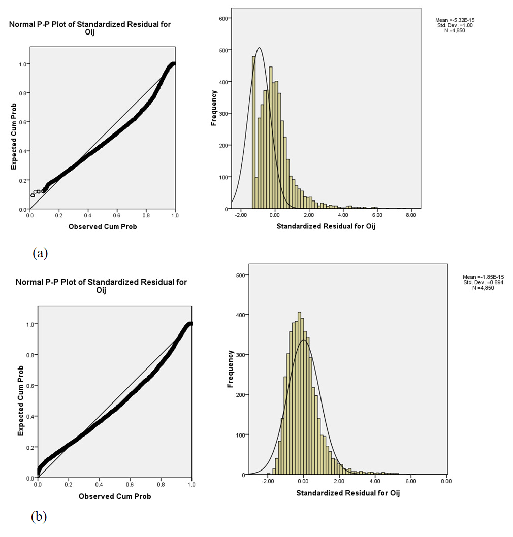
Figure 1: Residual plot and histogram for checking the normality assumption in the (a) one-factor ANOVA and (b) repeated measures model for the Economic sectors difference data analyzed in Section 4.1.
Table 2: Multiple comparisons under the Kruskal Wallis test for the Economic sectors difference data analyzed in Section 4.1, where * represents significant differences at a 0.05 level. The sample size is large and the design is balanced, thus the same normal approximation with mean 470450 and standard deviation 12336.55 can be used for each difference. Hence, the associated standardized statistics (in parentheses) can be compared with -1.96 and 1.96 at a 0.05 significance level.
| Difference | U statistic | p-value | Group | Sum of ranks | 10*(p-value) |
|---|---|---|---|---|---|
| 1-2 | 452635.0 (-1.44) | 0.148 | 1 | 959200.0 | 1.48 |
| 2 | 923570.0 | ||||
| 1-3 | 458438.0 (-0.973) | 0.330 | 1 | 953397.0 | 3.30 |
| 3 | 929373.0 | ||||
| 1-4 | 442804.0 (-2.24) | 0.025 | 1 | 969031.0 | 0.25 |
| 4 | 913739.0 | ||||
| 1-6* | 401405.0 (-5.59) | < 0.05 | 1 | 1010430.0 | < 0.05 |
| 6 | 872340.0 | ||||
| 2-3 | 457230.5 (-1.07) | 0.284 | 2 | 928165.0 | 2.84 |
| 3 | 954604.5 | ||||
| 2-4 | 468115.0 (-0.19) | 0.850 | 2 | 943720.0 | 8.50 |
| 4 | 939050.0 | ||||
| 2-6* | 402365.5 (-5.52) | < 0.05 | 2 | 1009469.5 | < 0.05 |
| 6 | 873300.5 | ||||
| 3-4 | 442457.0 (-2.27) | 0.023 | 3 | 969378.0 | 0.23 |
| 4 | 913392.0 | ||||
| 3-6* | 382866.5 (-7.10) | < 0.05 | 3 | 1028968.5 | < 0.05 |
| 6 | 853801.5 | ||||
| 4-6* | 386476.0 (-6.81) | < 0.05 | 4 | 1025359.0 | < 0.05 |
| 6 | 857411.0 |
In this sample, we have five observations for each s.u. whose values are related because they correspond to the same individual, i.e. s.u., so that it is more convenient to fit a repeated measures model. Then, variable O ij in (2) corresponds to the localization ratio in sector j, or population j, with j = 1, … , k, k = 5, for s.u. i; i = 1, …, L; L = 970, I corresponds to the s.u. effect, and S to the sector effect.
We determined after fitting model (2) that there is effect of sector (F = 11.27, p-value < 0.05, critical value =
Table 3: ANOVA for the two-factor model representing a repeated measures model for the Economic sectors difference data analyzed in Section 4.1. Critical value is 2.37 at a 0.05 significance level.
| Source | SS | df | Mean Square | F | p-value |
|---|---|---|---|---|---|
| Sector | 43.553 | 4 | 10.888 | 11.265 | < 0.05 |
| S.u. | 241.593 | 969 | 0.249 | ||
| Error | 3746.493 | 3876 | 0.967 | ||
| Total | 4031.640 | 4849 |
Table 4: Univariate and multivariate tests to determine effect of sector on the localization ratio for the Economic sectors difference data analyzed in Section 4.1. Critical values for each test can be calculated from a F distribution with the numerator df obtained from the part in which source is Sector and the denominator df obtained from the part in which source is Error, e.g. F 0.95 (4,3876) = 2.37 for sphericity at a 0.05 significance level.
| Univariate | Multivariate | |||||||||
|---|---|---|---|---|---|---|---|---|---|---|
| Source | SS | df | MS | F | p-value | Test | Value | F | p-value | |
| Sector | Sphericity assumed | 43.553 | 4.00 | 10.888 | 11.265 | < 0.05 | Pillai’s Trace | 0.056 | 14.281 | < 0.05 |
| Greenhouse- Geisser | 43.553 | 2.91 | 4.992 | 11.265 | < 0.05 | Wilks’ Lambda | 0.944 | 14.281 | < 0.05 | |
| Huynh-Feldt | 43.553 | 2.91 | 14.942 | 11.265 | < 0.05 | Hotelling’s Trace | 0.059 | 14.281 | < 0.05 | |
| Lower-bound | 43.553 | 1.00 | 43.553 | 11.265 | 0.001 | Roy’s Root | 0.059 | 14.281 | < 0.05 | |
| Error | Sphericity assumed | 3746.493 | 3876.00 | 0.967 | ||||||
| Greenhouse- Geisser | 3746.493 | 2815.12 | 1.331 | |||||||
| Huynh-Feldt | 3746.493 | 2824.49 | 1.326 | |||||||
| Lower-bound | 3746.493 | 969.00 | 3.866 | |||||||
Table 5: Multiple comparisons for the Economic sectors difference data analyzed in Section 4.1 under the repeated measures model and considering spatial units as a random factor, where * represents significant differences at a 0.05 level. For the repeated measures model, the critical values at the same level are t 0.95 3876 = 1.961 and -1.961 (two sided test), which must be compared with the estimated difference divided by its standard error. For the random effects model, the procedure is similar, but the critical values are t 0.95 4845 = 1.960 and -1.960.
| Repeated measures model | Random effect | |||||||
|---|---|---|---|---|---|---|---|---|
| Diference | Estimated value |
Std. Error | p-value | 95% Condidence interval |
Estimated value |
Std. Error | p-value | |
| 1-2 | 0.145* | 0.047 | 0.002 | 0.053 | 0.236 | 0.145* | 0.045 | 0.001 |
| 1-3 | 0.217* | 0.043 | < 0.05 | 0.133 | 0.301 | 0.217* | 0.045 | < 0.05 |
| 1-4 | 0.284* | 0.041 | < 0.05 | 0.203 | 0.364 | 0.284* | 0.045 | < 0.05 |
| 1-6 | 0.135* | 0.059 | 0.023 | 0.018 | 0.252 | 0.135* | 0.045 | 0.002 |
| 2-3 | 0.072* | 0.035 | 0.039 | 0.004 | 0.141 | 0.072 | 0.045 | 0.105 |
| 2-4 | 0.139* | 0.034 | < 0.05 | 0.073 | 0.205 | 0.139* | 0.045 | 0.002 |
| 2-6 | -0.010 | 0.054 | 0.860 | -0.115 | 0.096 | -0.010 | 0.045 | 0.831 |
| 3-4 | 0.067* | 0.022 | 0.003 | 0.023 | 0.110 | 0.067 | 0.045 | 0.136 |
| 3-6 | -0.082 | 0.049 | 0.098 | -0.179 | 0.015 | -0.082 | 0.045 | 0.067 |
| 4-6 | -0.148* | 0.050 | 0.003 | -0.247 | -0.050 | -0.148* | 0.045 | 0.001 |
Observe that the residuals in model (2) (Figure 0) are closer to a normal distribution than those in model (1) (Figure 1(b)), even though, according to a Lilliefors’ test, normality is rejected (test statistic = 5.27, p-value < 0.05, critical value = 1.36). Observe also that in model (2) we considered individual as a fixed effect; however, as individuals are part of a random sample, we could consider it as a random effect, see e.g. (Lindsey, 1999, p. 89). Thus, we fitted a mixed effects model and obtained results which are in close agreement with those from the repeated measures model. There is effect of sector (F test with F = 11.25; p-value < 0.05, critical value =
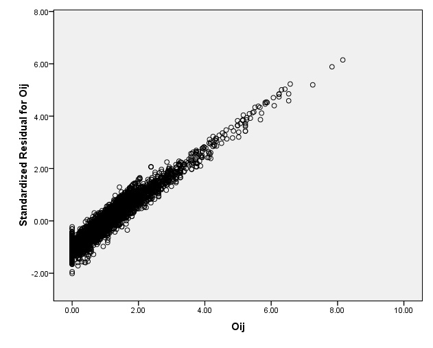
Figure 2: Residual plot for checking the homoscesdaticity assumption in the repeated measures model for the Economic sectors difference data analyzed in Section 4.1.
Using a significance level of 0.05, we rejected the null hypothesis corresponding to the Friedman test (test statistic = 85.71 with 4 d.f., p-value < 0.05, critical value =
Table 6: Multiple comparisons under the Friedman test for the Economic sectors difference data analyzed in Section 4.1, where * represents significant differences at a 0.05 level. Since Z is a standardized score, at a 0.05 significance level, the critical value for each difference is -1.96 and 1.96 (two-sided test).
| Difference | Z score | p-value | Ranks | Sum of ranks | 10*p-value |
|---|---|---|---|---|---|
| 1-2 | -1.956 | 0.050 | Negative | 205293.00 | 0.50 |
| Positive | 237918.00 | ||||
| 1-3 | -2.430 | 0.015 | Negative | 207085.00 | 0.15 |
| Positive | 248450.00 | ||||
| 1-4* | -4.254 | < 0.05 | Negative | 197060.00 | < 0.05 |
| Positive | 270968.00 | ||||
| 1-6* | -4.428 | < 0.05 | Negative | 173326.00 | < 0.05 |
| Positive | 243915.00 | ||||
| 2-3 | -0.311 | 0.756 | Negative | 227971.00 | 7.56 |
| Positive | 233309.00 | ||||
| 2-4 | -1.948 | 0.051 | Negative | 218465.00 | 0.51 |
| Positive | 252470.00 | ||||
| 2-6* | -2.954 | 0.003 | Negative | 193109.00 | 0.03 |
| Positive | 241669.00 | ||||
| 3-4* | -3.295 | 0.001 | Negative | 206273.00 | 0.01 |
| Positive | 263692.00 | ||||
| 3-6* | -2.962 | 0.003 | Negative | 201678.00 | 0.03 |
| Positive | 251950.00 | ||||
| 4-6 | -2.106 | 0.035 | Negative | 216626.00 | 0.35 |
| Positive | 253339.00 |
Simulation
The importance of selecting an adequate test was studied through simulated data. A sample corresponding to three repeated correlated measures is obtained and we see that the error and inference associated vary according to the model and assumptions used. Three random samples of size 1000, a size similar to the one in the data, based on a normal distribution with mean zero and variance σ2 = 0.5 setting a fixed seed were obtained. For the first sample we added 1.5 to the normal distribution. The second and third samples corresponded to multiply the normal distribution by 0.65 and 0.9, respectively, and after that, the same value of 1.5 was added. Hence, all three samples have mean 1.5. It can also be seen that by construction all three samples are perfectly correlated, so that they are not independent between them. This is because for instance
for X a random variable whose distribution is normal and b a constant term (0.65 or 0.9). As a consequence, the associated correlation
whereas, between the first and third populations we have
By not assuming sphericity, we infer that the samples have the same mean (F = 3.14, p-value < 0.08, critical value =
To measure errors associated with the simulation, 100 simulations were conducted, that is, we obtained 100 data sets formed each by three correlated random samples according to the same scheme described before. The Mean Squared Error (MSE) associated with the mean for each of the three correlated measures, considering the real mean, 1.5, and the sample mean Yij in each data set i = 1,...,100, for each of the three measures j, j = 1,2,3, can be obtained as
For the first sample, in which the random variable X is not multiplied by any term, the MSE has a value of 0.0238. For the second and third samples, whose associated random variable is multiplied by 0.65 and 0.9, respectively, the MSE corresponded to 0.0154 for the former and 0.0214 for the latter samples. For each of the 100 simulated data sets, the estimated coefficients under a one-factor ANOVA can be obtained, in particular, the estimated constant term (global mean). The standard error between simulations associated with any estimated coefficient
where
The same process can be followed for the repeated measures model considering sphericity. In this case the standard error between simulations associated with the constant term is 0.603, which is larger since terms concerning each observation are included in the model. The proportion of the simulated data sets whose p-value is less or equal than 0.05 is 9% (or 12% using a 0.1 significance level). This means that in some cases, as in the sample shown above, it is erroneously inferred that the sample mean is the same between the three correlated samples, which occurs because the variance structure is not properly modeled.
Income difference between three different types of localities
To determine whether the distribution of income is the same between all three types of regions in the Income difference data introduced in Section 2, we used an one-factor ANOVA in which income I and type of locality L are the dependent and independent variables, respectively. There is a significant difference of income between the three types of regions (F test with F = 1308.63, p-value < 0.05, critical value =
After fitting the transformed model, we observed that both the normality and homoscedasticidity of the residuals assumptions were improved. For the former, we can see from the associated PP-plot (Figure 3(b)) that residuals are closer to the 45o straight line, and for the latter we did not reject homoscedasticity according to Levene’s test (Levene’s W = 0.25, p-value < 0.78, critical value =
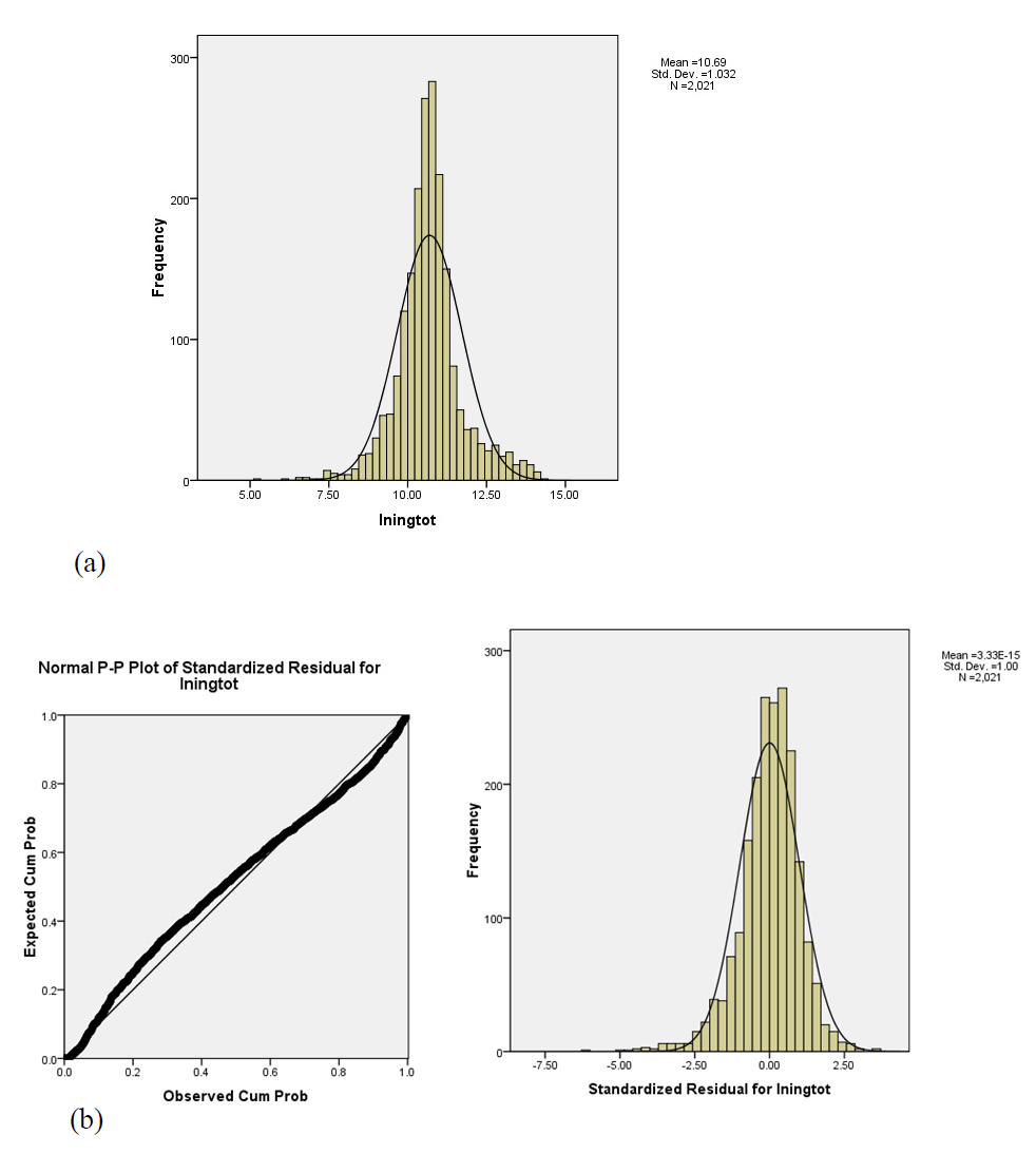
Figure 3: (a) Histogram for the transformed income variable and (b) residual plot and histogram for checking the normality assumption in a one-factor ANOVA using the transformed variable for the Income difference data analyzed in Section 4.2.
Table 8: Multiple comparisons under the one-factor ANOVA and GWR model for the Income difference data analyzed in Section 4.2, all differences are significant (*) at a 0.05 level. At the same level the critical values associated with the one-factor ANOVA are t 0.975 2018 = 1.961 and -1.961, which should be compared with the estimated difference divided by its standard error (in parentheses). For the GWR model the critical value is LSD 0.05 .
| One-factor ANOVA | GWR model | ||||||
|---|---|---|---|---|---|---|---|
| Diference | Estimated value |
Std. Error | p-value | 95% Interval | Estimated |
LSD 0.05 | |
| Urban-Periurban | 2.126 (26.66)* | 0.0797 | < 0.05 | 1.939 | 2.312 | 2.653* | 0.139 |
| Urban-Rural | 2.681 (33.60)* | 0.0798 | < 0.05 | 2.494 | 2.869 | 2.108* | |
| Periurban-Rural | 0.556 (14.78)* | 0.0380 | < 0.05 | 0.468 | 0.644 | 0.545* | |
Each observation in this example corresponds to a s.u., and, as a consequence, the dependent variable might be spatially correlated. We obtained the projected coordinates for each s.u, then we calculated the Moran’s I associated with both the dependent variable and the residuals associated with the corresponding one-factor ANOVA. Because we are working on a sample of spatial units, we determined the neighbors set and calculated the spatial weights using k nearest neighbors with k = 5. For the dependent variable, Moran’s I takes a value of 0.26 and we significantly reject that there is no spatial autocorrelation (p-value < 0.05, standardized Moran’s I = 19.76, assuming normality critical values are -1.96 and 1.96 at a 0.05 significance level). This means that units with high income are closer to units with high income and similarly for those with low income (recall that we are actually working with income in a logarithmic scale). For the residuals corresponding to the one-factor ANOVA, we got a significant Moran’s I of 0.28 (p-value < 0.05, standardized Moran’s I = 21.62, assuming normality critical values are -1.96 and 1.96). This means that the independence assumption is violated because of spatial dependence. As a consequence, fitting a GWR model which considers such dependence may be a better option.
We fitted a GWR, where the logarithm of income is the dependent variable and type of region L is an independent variable. Note that when a GWR is fitted, we actually obtain an estimated parameter for each s.u., so that we only show the minimum, maximum, and median corresponding to such parameters (Table 7). By analyzing the median, we see that the parameters estimated under the GWR model are similar to those obtained through the one-factor ANOVA (Table 7). The parameters imply that compared with periurban regions in urban regions there is a higher income and that in rural regions there is a lower income, both in a logarithmic scale. A global determination coefficient can be obtained, it takes a value of 0.61, which is greater than the one obtained for the one-factor ANOVA (0.37). The estimated standard deviation takes a value of 0.65, so that it decreased compared to the other model (0.82). Using the residuals, we calculated Moran’s I and it takes a significant value of 0.05 (p-value < 0.05, standardized Moran’s I = 3.78, assuming normality critical values are -1.96 and 1.96), which is close to zero, so that by fitting a GWR model, spatial autocorrelation was eliminated and the independence assumption is satisfied.
Table 7: Parameter estimates for the one-factor ANOVA and GWR model for the Income difference data analyzed in Section 4.2. For the one-factor model, the critical values (two-sided test) to test parameter significance can be obtained from quantile t 0.975 2018 = 1.961 at a 0.05 significance level (it should be compared with t, third column).
| One-factor ANOVA | GWR estimators | ||||||||
|---|---|---|---|---|---|---|---|---|---|
| Parameter | β | Std. Error | t | p-value | 95% Interval | Min | Median | Max | |
| Intercept | 10.828 | 0.026 | 408.752 | < 0.05 | 10.776 | 10.880 | 10.010 | 10.820 | 12.490 |
| Periurban | 0 | - | - | - | - | - | - | - | - |
| Urban | 2.126 | 0.080 | 26.659 | < 0.05 | 1.969 | 2.282 | 0.263 | 2.153 | 3.376 |
| Rural | -0.556 | 0.038 | -14.778 | < 0.05 | -0.630 | -0.482 | -2.211 | -0.485 | 0.397 |
Once fitting this model, we can perform a post hoc analysis. This analysis is not directly available; however, we calculated the estimated means under the GWR by using the estimated values; and through them, we performed multiple comparisons by using Tukey’s honestly significant differences. That is, from the estimated values, we calculated the estimated means for each region
in which LSD α is the honestly significant difference at a significance level α
where MSE is the mean square error, which can be replaced by the unbiased variance estimator;
with n i the number of units in region i, i = 1, 2, 3 and t = 3.
Using a significance level of 0.05, the second part in equation (4), the critical value LSD α , takes a value of 0.139. All estimated means differences are greater than this value, so that we reject that each pair of populations has the same mean under the GWR model. Once again, the order of income according to the type of region is the same as before (Table 8).
Discussion
The equivalence between models and methods to test whether the distribution of a variable is the same between populations or groups was presented. According to the lack or not of the normality assumption parametric or non-parametric methods can be used. When data correspond to geographical information, there are some of these analyses that are more adequate because their assumptions are closer to reality because they account for spatial dependency or autocorrelation. We presented and compared these methods and models in general and in the context of geographical data.
The one-factor ANOVA is presented as the most basic linear model to test whether the mean of a variable is the same between populations; it can be expressed as a linear model whose associated assumptions are inherited from linear regressions. It is a parametric method. The analogous non-parametric test corresponds to the Kruskal-Wallis one. When several variables are measured for the same individual; for instance the same spatial unit, we test whether the distribution is the same in each measure using a repeated measures model in the parametric case and a Friedman test in the non-parametric case. Parametric methods can be seen as linear models whose associated tests are related with the means in each population. A repeated measures model can be expressed as a two-factor ANOVA, including individual as an explanatory variable, when the sphericity assumption is considered. This factor can be considered as fixed or random, the last case being a mixed model. In all cases, once rejecting the null hypothesis concerning similar distributions or means between populations accordingly, a post hoc analysis can be performed allowing to identify the populations where there is a significant difference. We showed the relationships between all methods and the assumptions concerning each one.
We applied all four methods when data concerning spatial units are involved. We analyzed in specific regions in Mexico that are neither urban non rural according to their population size, whether the localization ratio was similar between five economic sectors. This means that all sectors are equally important in such regions. We rejected such economic similarity and found evidence that the Construction sector has the highest values. The model and test that seem more adequate considering assumptions and suitability of the methods themselves were the repeated measures model and Friedman test. We showed through simulated observations how a model considering assumptions not satisfied by the data can lead to wrong conclusions and how an adequate model can decrease the associated error. Because all economic sectors are not equally important, it makes sense to measure economic diversity through an entropy index. We are currently calculating it and obtaining the associated maps to identify whether there are the regions in Mexico where all sectors are equally relevant.
When we want to compare means between populations in data concerning spatial information, independence can be violated when the information is spatially related; this may happen for instance when a one-factor ANOVA is used in spatial data. This implies that a model including such dependence is preferred. A model of this kind can be obtained from a geographically weighted regression (GWR), which depends on the geographical coordinates associated with each observation and includes a variable that separates populations as a factor. After fitting a GWR model the independence assumption should be satisfied. As in a one-factor ANOVA, multiple comparisons can be obtained, even if the software does not perform them. We obtained them using Tukey’s honestly significant differences.
We illustrated the use of a GWR analogous to a one-factor ANOVA through an analysis of data concerning income in a logarithmic scale for spatial units in three different regions in Mexico: urban, rural, and those that are neither rural nor urban. When an ANOVA was used, the independence assumption was violated because income is spatially related, after fitting an analogous model but using a GWR this was fixed. We observed that there is a significant difference in the income between regions and that there are significantly highest values in urban regions followed by those territories that are neither rural nor urban, while the lowest values correspond to rural regions.
Additional work corresponds to include the spatial dependence in more advanced models than a one-factor ANOVA; for instance, in a repeated measures model. In such models, we would be considering the dependence there is between observations taken in the same spatial unit and between the spatial units; the latter is not considered in an usual repeated measures model. The simplest case would be when the sphericity assumption is considered. In this case we could use a GWR equivalent to a two-factor ANOVA, that is, a model including the spatial unit as a fixed factor together with another factor that divides the data into populations. It could be even more interesting to try to implement a geographically dependent model equivalent to a repeated measures model in which sphericity is not assumed. That is, to try to generate tests as the multivariate ones or the Greenhouse-Geisser correction for a repeated measures model that is spatially dependent. There are other linear models besides GWR that consider dependence between spatial units (spatial autocorrelation); for instance, spatially lagged y models, see (Ward and Gleditsch, 2008). We could try to use these models instead to define an ANOVA with spatial dependence as the one used in Section 4.2.

