Introduction

Dynamical systems is one of the most interesting mathematical areas, whose development has been accelerated by the increasing computing power in the last decades. Since Lorenz's meteorological model (^{Lorenz, 1963}), or Chen’s (^{Chen and Ueta, 1999}) and Lü’s (^{Lü and Chen, 2002}) models, these systems have captured the attention to analyse their dynamic properties.

The simplest dynamical system families that show chaotic behavior are autonomous dynamical systems in three dimensions with quadratic nonlinearities (^{Malihe, et al., 2013}). There are some examples, such as the Lorenz chaotic system and others, where their equilibrium points are unstable and none of them has more than three. Recent studies have been conducted in systems containing stable equilibria and yet show chaotic behavior (^{Sprott, 1993}, ¹⁹⁹⁴, ¹⁹⁹⁷, ²⁰⁰⁰).

In (^{Wang and Chen, 2012}) it is shown how to build some simple chaotic systems that can have any number of equilibria. The constructed new systems exhibit chaotic behavior, regardless of the number of equilibria. In addition, it is included a review of some of Sprott's chaotic systems with a single equilibrium. For Sprott's D and E systems, degenerated equilibria are obtained, and a small perturbation intends to lead these systems with degenerated equilibria to stable points. The procedure consists in including a constant control parameter, trying to change the stability of its single equilibrium point to a stable one, while preserving its chaotic dynamics.

It is noticeable that by changing the constant control parameter the unstable equilibrium changes from a saddle point to a node, while the chaotic dynamics survives in a narrow range of the parameter. As the new system is not hyperbolic, the homoclinic Shilnikov criterion is not applicable. Nevertheless, the new system is chaotic in the following sense: it has a positive Lyapunov exponent, a fractional dimension, a continuous frequency spectrum and a period- doubling behavior route to chaos.

In (^{Malihe et al., 2013}), twenty-three chaotic systems are presented. Each three-dimensional autonomous system with quadratic nonlinearity has a single equilibrium point that is stable according to the Routh-Hurwitz criterion. These systems belong to a class of chaotic systems with a hidden attractor. It is also shown that chaotic jerk systems with quadratic nonlinearities cannot have multiple stable equilibria. Furthermore, it is proven in the same article that for any polynomial jerk system all the equilibria cannot be simultaneously stable.

In (^{Sajad and Sprott, 2013}) nine chaotic systems with quadratic nonlinearities are presented, and they are characterized by having a straight line as their respective equilibrium. Those systems are a class of chaotic systems with hidden attractors as already mentioned. It is shown that all the cases have a stable equilibrium, and an attractor point coexists with a strange attractor.

^{Sifeu et al. (2013)} present a three-dimensional autonomous chaotic system and its physical implementation. By adjusting the respective parameters, the system exhibits periodic and chaotic oscillations similar to the heart sound signals. The system contains heteroclinic orbits in the sense of Shilnikov, therefore it is concluded that the three-dimensional system presents horseshoe-type chaos.

The aim of this paper is to report ten new simple nonlinear autonomous quadratic systems in three dimensions, which have one asymptotically stable equilibrium point and chaotic behavior. These new systems were found mainly by the use of the Monte Carlo method. Previously, the Monte Carlo method was used in (Carrillo et al., 2013) and recently in (^{Sprott and Xiong, 2015}) for similar purposes. These systems belong to a family of hidden attractors. There are few systems like these presented here reported in the current literature, being interesting due to their difficult search and unusual properties.

To justify the chaotic dynamics for these systems, Lyapunov exponents and Kaplan-Yorke dimensions were calculated. Bifurcation diagrams and phase portraits are also shown. It can be seen in the phase portraits of each model, both chaotic behavior as well as asymptotically stable equilibrium points.

We found that these systems contain a hidden attractor due their behavior. An attractor is called hidden attractor if its basin of attraction does not intersect with small neighborhoods of equilibria, Otherwise it is called self-excited attractor (^{Leonov and Kuznetsov, 2013}). The chaos of these systems is not defined in the sense of Shilnikov or Smale.

2. Preliminaries

In this section, definitions and theorems are presented to analyze the behavior of the orbits of the proposed systems. The first definition describes the local stability of a system having an hyperbolic saddle focus; the second definition is about the homoclinic trajectories of a system and the third describes the case when a system has heteroclinic orbits.

Let us consider an nth-order autonomous system:

(1)

where the vector field f = (f ₁ , f ₂ , f ₃ ,..., f _n ) ^T : Rⁿ → Rⁿ belongs to class C ^r (r≥1) and x = (x ₁ , x ₂ , x ₃ ,..., x _n ) ^T is the state variable of the system, and t є R is the time. Suppose that f has at least one equilibrium point P.

Definition 1. (^{Elhadj and Sprott, 2012}) The point P = (p ₁ , p ₂ , p ₃ ,..., p _n ) is called a hyperbolic saddle focus for system (1) if the eigenvalues of the Jacobian A = Df( x ), evaluated at P, are γ and α+βi, where αγ<0 and β≠0.

Definition 2. (^{Elhadj and Sprott, 2012}) A homoclinic orbit γ (t) refers to a bounded trajectory of the system (1) that is doubly asymptotic to an equilibrium point P of the system, i.e., lim _t→-∞ γ (t)= lim _t→+∞ γ (t)=P.

The next definition requires the existence of at least two equilibrium points P ₁ and P ₂ .

Definition 3. (^{Elhadj and Sprott, 2012}) A heteroclinic orbit δ (t) is similarly defined as in Definition 2, except that there are two distintic saddle foci P ₁ and P ₂ connected by the orbit, one corresponding to the forward asymptotic time, and the other to the reverse asymptotic time limit, i.e., lim _t→+∞ δ(t)=P ₁ and lim _t→-∞ γ(t)=P ₂ .

Theorem 1 characterizes the conditions under which a system does not present homoclinic or heteroclinic orbits. From this information we can identify systems that present Smale's horseshoe behavior. It is important to note systems that exhibit behaviors such as Smale's horseshoe when they have a hyperbolic saddle focus. For systems that do not contain this hyperbolic saddle focus their chaotic behavior is not in the sense of Shilnikov.

Theorem 1. (^{Elhadj and Sprott, 2012}) Suppose that there exists at least one integer j є {1, 2, 3,..., n} such that the component fj( x ) satisfies that there exists α<0: fj( x )≥α, Ɐx є Rⁿ. Then the system (1) cannot have homoclinic and heteroclinic orbits.

Definition 4. (^{Perko, 1991}) An equilibrium a of d x /dt = f( x ) is called hyperbolic if none of the eigenvalues of Jacobian Df(a) has real part 0.

Theorem 2. (^{Perko, 1991}) Let a be an equilibrium of d x /dt= f( x ) . If the real part of each eigenvalue of Df(a) is strictly negative, then a is asymptotically stable. If the real part of at least one eigenvalue is strictly positive, then a is unstable.

Definition 4 and Theorem 2 serve to study the local stability in nonlinear systems. In the next section we present ten new chaotic systems. The definitions and theorems presented in this section will be used later on to analyze the systems we report in this paper.

3. Chaotic systems with an asymptotically stable equilibrium point.

These new three-dimensional nonlinear autonomous systems with quadratic nonlinearities are listed in Table 1. Unlike other systems reported in the literature, these systems have different characteristics. This article is based in the following system of differential equations:

(2)

where: X = (x, y, z) ^T , R = (yz, xz, xy) ^T and S = (x ² , y ² , z ² ) ^T , are the vectors of the state variables, the cross products and quadratic terms of the state variables of the system, respectively. The parameters are: A ₀ = (a ₁ , a ₂ , a ₃ ) ^T , M = (m _ij ), N = (n _ij ) y Q = (q _ij ), for Ɐi = 1, 2, 3, Ɐj = 1, 2, 3.

Table 1 Models 

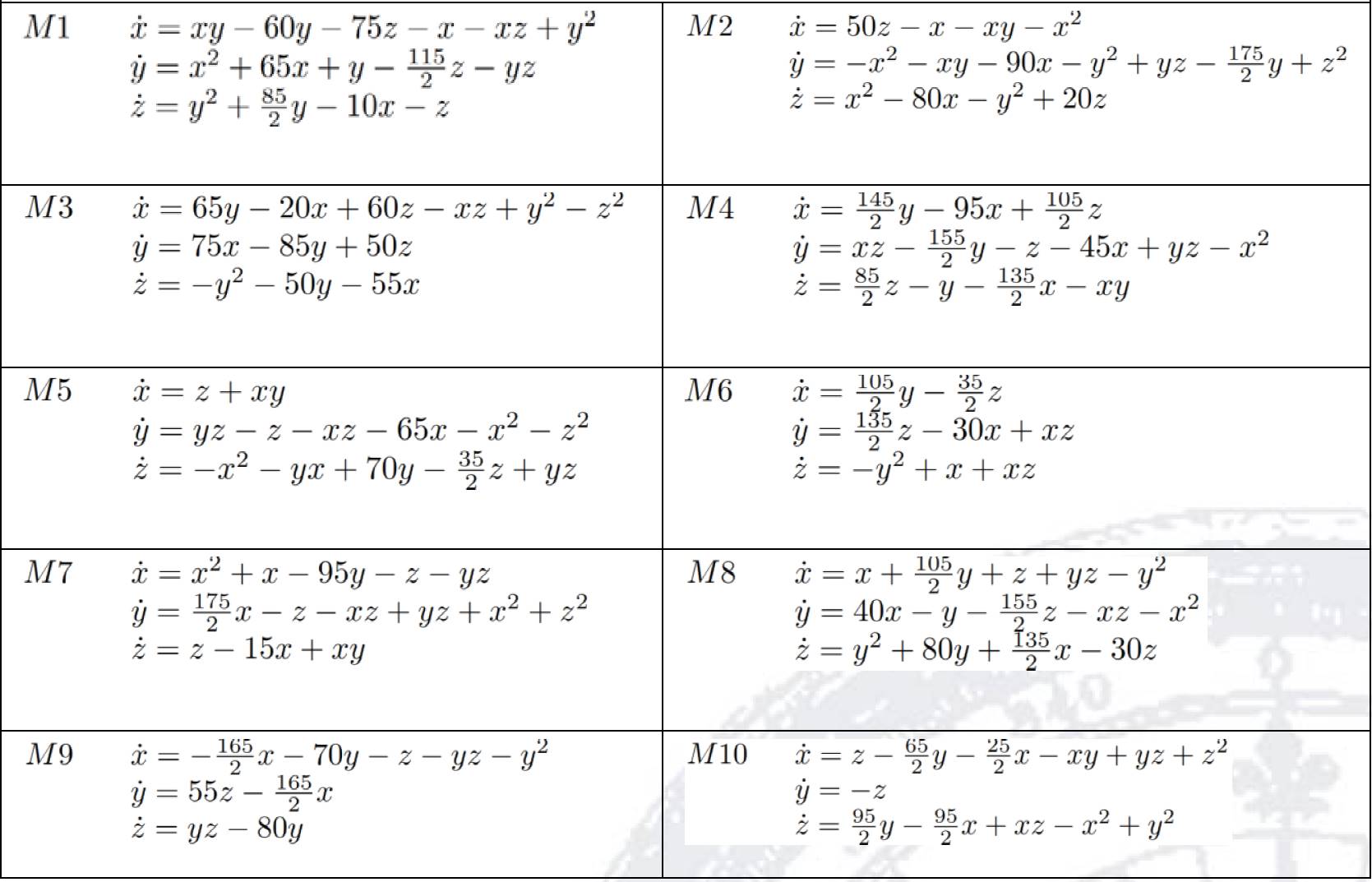
The methodology to generate new systems is by using the Monte Carlo method (^{Press et al., 1996}). We generate values for the parameters in equation (2) in order to randomly generate a new system as we set A₀ = (0, 0, 0). The elements of M are set within the range [-100; 100] with a length step of 2.5 and it includes the possible values of {-1, 1} and the elements of N and Q are only set to {-1, 0, 1}.

For each point in the randomized set, the corresponding equation is solved using a fourth-order fixed-step Runge-Kutta method. The Lyapunov exponents are calculated and if there is an exponent greater than 0.5 the system is chosen.

It is important to say that the use of Monte Carlo method is only to search for new systems. The systems where one of their exponents is positive are consider as chaotic systems. The chaotic systems found are shown in Table 1.

As we can see in Table 1, the systems are not symmetrical and each differential equation contains at least one quadratic term accompanied by one or more cross terms, unlike the aforementioned systems reported in (^{Malihe, 2013}).

Table 2 presents the synthesis of the ten models, their Lyapunov exponents (LEs), the asymptotically stable equilibrium point (Eq) of each one of them and the eigenvalues of the system at its asymptotically stable equilibrium point (Eig).

Table 2 Systems’ Description 

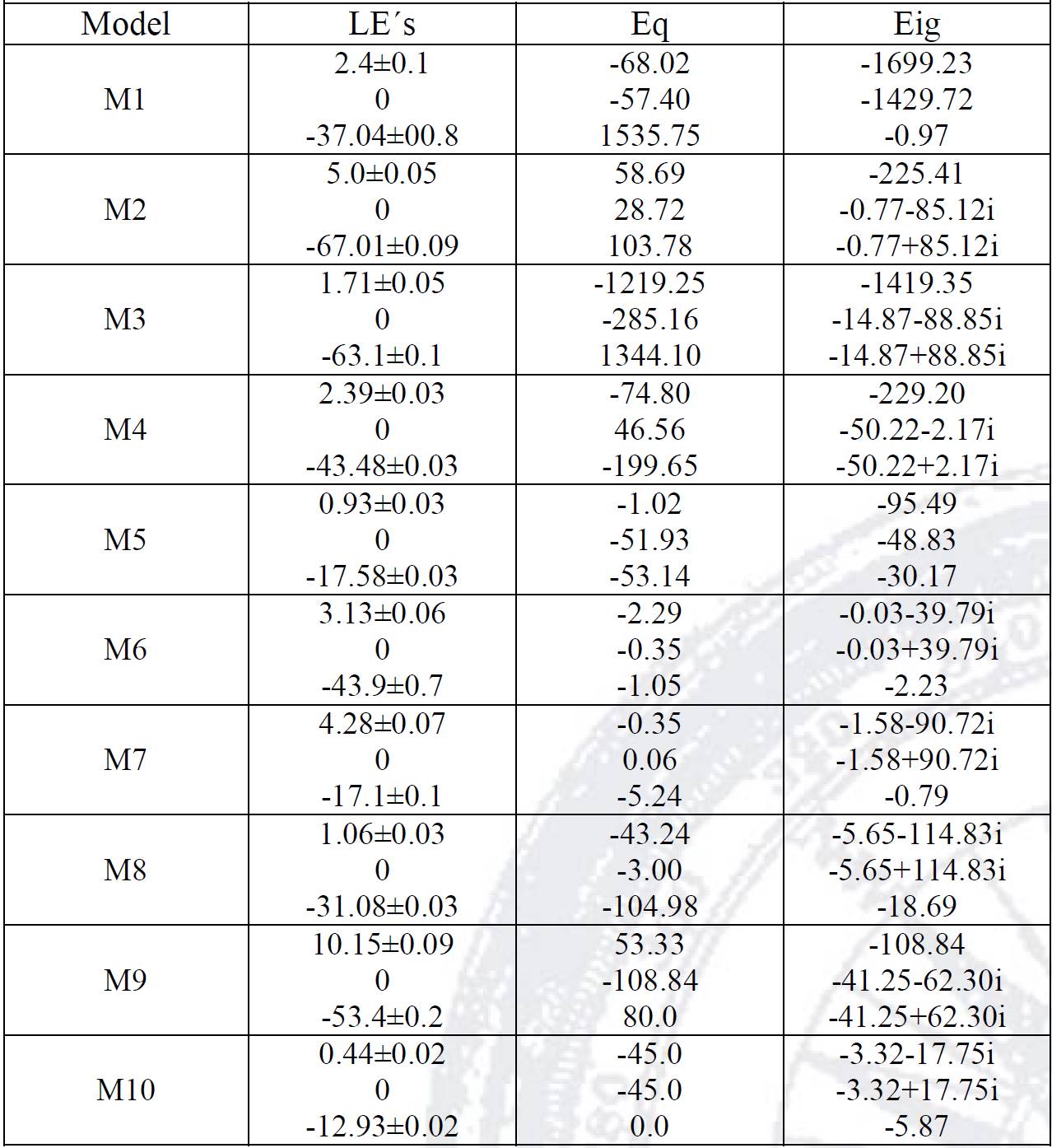
The names of the systems are placed in the first column of Table 2. In the second column, the Lyapunov exponents are reported for each model, with an error term. To construct this result, 100 different random initial conditions were taken to calculate the root mean square error to find a bound for the possible error in the Lyapunov exponents. To calculate Lyapunov exponents a Runge-Kutta integrator was used with an adaptive step size and 1000 time units.

In the third column of Table 1, it is reported just one equilibrium point for each system and in the fourth column the eigenvalues of the equilibrium point taken from the third column are shown. To create phase portraits for the systems M1, M2, M4, M5, M6, M7, M8, M9 and M10 the initial condition [1, 1, 0] was used. For the system M3, the initial condition was [1, 1, 1].

From Table 2 we can highlight the following results. The most important characteristic of the models presented is that all of them have an asymptotically stable equilibrium. Although we have local stability in all cases, the models have a positive Lyapunov exponent, which suggests a chaotic behavior.

In Table 3 the equilibria of the ten systems are presented. Some of them containing up to 7 equilibria, as the case of M1, but others have only 3 points of such type. The left column (Eq) shows the equilibria, and the right column (Eig) shows the corresponding eigenvalue at that point. All equilibrium points are hyperbolic systems. M1, M5 and M7 are those systems which contains more equilibria. On the other side, M6 and M9 are those with fewer equilibria.

Table 3 Equilibrium Points of Systems 

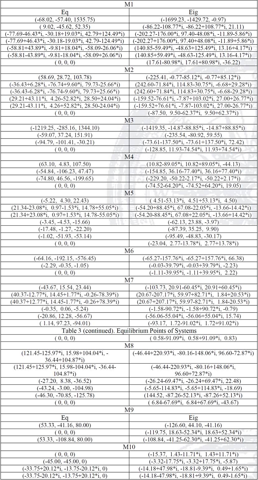
Definition 4 and Theorem 2 provide information with respect to the local stability of the models. Models M1 and M5 have all negative real eigenvalues, therefore they have a sink at a asymptotically stable point.

On the other hand, the rest of the models present one negative real eigenvalue and two complex conjugate eigenvalues with negative real part. Hence all these equilibria have an asymptotically stable spiral.

Figs. 1 to 10 show the bifurcation diagram and a trajectory in the phase space (R³) for each model. For the bifurcation diagrams of models M1, M6, M7 and M8 the parameter that was swept was m₁₂; models M3, M4, M9 and M10 used parameter m₁₁; model M2 uses parameter m₁₃ and model M5 uses parameter m₂₁.

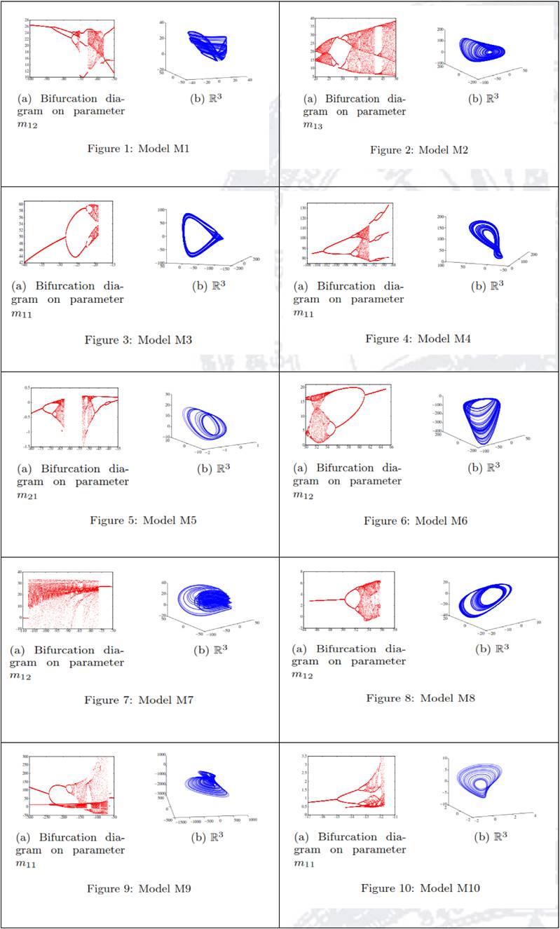
For models M1 (Fig. 1), M2 (Fig. 2), M3 (Fig. 3), M4(Fig. 4), M5 (Fig. 5), M6 (Fig. 6), M7 (Fig. 7), M8 (Fig. 8), M9 (Fig. 9) and M10 (Fig. 10), a period-doubling dependency on the variation of their respective parameter is presented while the chaotic behavior appears.

From Definitions 1-3 and Theorem 1 we know that the chaos presented is not of the Smale's horseshoe type due to the fact that the systems does not contain homoclinic or heteroclinic orbits and their equilibrium points are not saddle-focus.

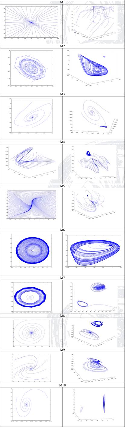
In Table 4 the phase portraits of the models are shown. For each model two subfigures are presented. On the left side the behavior of the asymptotically stable equilibrium is shown, while on the right subfigure, the chaotic behavior around a different equilibrium is presented.

Table no. 4 

There is a relationship between Lyapunov exponents and the Kaplan-Yorke dimension (^{Chlouverakis and Sprott, 2005}) given by:

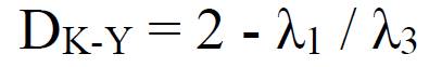(3)

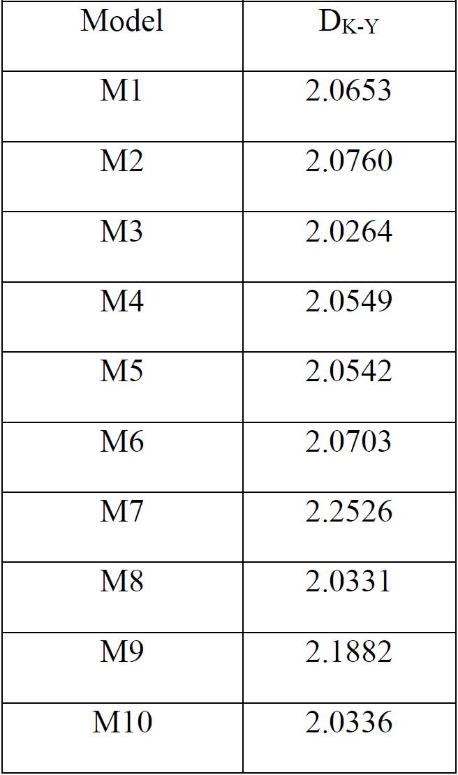
There is a wide variety of chaotic systems with dimensions that covers the range from 2 to 3. Most of these systems in the literature, as the Lorenz (^{Lorenz, 1963}), Lü (^{Lü and Chen, 2002}) and many others have only slightly larger than 2 Kaplan-Yorke dimension. In all our models the Kaplan-Yorke dimension is above 2, the largest Kaplan-Yorke dimension is found in model M7, as can be seen in Table 5.

Table 5: Kaplan-Yorke dimension for the ten models 

To conclude this section we highlight the following items. Systems reported by ^{Sprott (1994}, ¹⁹⁹⁷, ²⁰⁰⁰⁾ and ^{Wang - Chen (2012)} are nonlinear quadratic systems and for some cases rationals functions, with a single stable equilibrium and with chaotic behavior. These are a class of chaotic systems with a hidden attractor and with the property that they cannot have multiple stable equilibria.

Unlike the models mentioned above in this work, these systems are also chaotic, with only one asymptotically stable equilibrium point and containing a hidden attractor. These systems are ten new chaotic systems, which now are adding to those few systems known in the literature to this date.

The systems found by ^{Sprott (1993}, ¹⁹⁹⁴, ¹⁹⁹⁷, ²⁰⁰⁰) and ^{Wang - Chen (2012)} are not conjugates of the systems presented in this paper, i. e., the systems given by Sprott and Wang - Chen are not diffeomorphic with the systems that have been found in this work (^{Perko, 1991}).

4. Conclusions

In this paper, we have reported ten new quadratic nonlinear autonomous systems in three dimensions. We have obtained them by randomizing the parameter space through the Monte Carlo method. All systems shown have one asymptotically stable equilibrium point, but at the same time, all of them have evidence of chaotic behaviour. The asymptotic stability in these systems is a local property, coexisting with the global property determined by the chaotic behaviour of these systems.

Most of the models show double period chaos taking into account their bifurcation diagrams. The chaos behaviour of the studied systems is not of the class of Smale's horseshoe type, due to their orbits are not neither homoclinic nor heteroclinic in the sense Shilnikov.

The Kaplan-Yorke dimensión calculations of these systems also confirm a non-integer dimension, in concordance with others chaotic systems found in the literature.