


Servicios Personalizados
Revista
Articulo
 Inglés (pdf)
 Artículo en XML
 Referencias del artículo
 Enviar artículo por email
Indicadores
-
 Citado por SciELO
 -
 Accesos
Links relacionados
-
 Similares en
SciELO
Similares en
SciELO
Compartir

 Permalink
Nova scientia
versión On-line ISSN 2007-0705
Nova scientia vol.6 no.12 León oct. 2014
Ciencias Naturales e Ingenierías
Modified nonlinearities distribution Homotopy Perturbation method as a tool to find power series solutions to ordinary differential equations
Método modificado de Perturbación Homotópica con distribución de no linealidades como herramienta para encontrar soluciones de ecuaciones diferenciales ordinarias
U. Filobello-Nino1, H. Vázquez-Leal1, Y. Khan2, D. Pereyra-Díaz1, A. Pérez-Sesma1, A. Díaz-Sánchez3, V.M. Jiménez-Fernández1, A. Herrera-May4, R. López-Martínez5 and J. Sanchez-Orea1
1Electronic Instrumentation and Atmospheric Sciences School, University of Veracruz, Xalapa, Veracruz
2 Department of Mathematics, Zhejiang University, China
3 National Institute for Astrophysics, Optics and Electronics, Puebla
4 Micro and Nanotechnology Research Center, University of Veracruz, Veracruz
5Mathematics School, University of Veracruz, Xalapa, Veracruz
Uriel Filobello-Niño. E-mail: ufilobello@gmail.com
Recepción: 25-06-2013
Aceptación: 03-12-2013
Resumen
En este artículo, el método modificado de perturbación homotópica con distribución de no linealidades (MNDHPM) es utilizado para encontrar soluciones en series de potencias de ecuaciones diferenciales ordinarias, tanto lineales como no lineales. Se verá que el método es particularmente relevante en algunos casos de ecuaciones con coeficientes no polinomiales e inhomogéneas con términos no homogéneos no polinomiales.
Palabras clave: ecuaciones diferenciales, soluciones en series de potencias, Método de perturbación homotópica, Método de perturbación homotópica con distribución de no linealidades, Métodos aproximados.
Abstract
In this article, modified non-linearities distribution homotopy perturbation method (MNDHPM) is used in order to find power series solutions to ordinary differential equations with initial conditions, both linear and nonlinear. We will see that the method is particularly relevant in some cases of equations with non-polynomial coefficients and inhomogeneous non-polynomial terms.
Keywords: differential equations, power series solutions, Homotopy perturbation method, Homotopy perturbation method with no linearities distributions, approximate methods.
1. - Introduction
As widely known, the importance of research on nonlinear differential equations is that many phenomena, practical or theoretical, are of nonlinear nature. In recent years, several methods focused to find approximate solutions to nonlinear differential equations, as an alternative to classical methods, have been reported, such those based on: variational approaches (Kazemnia et al. 2008; Noorzad et al. 2008), tanh method (Evans and Raslan 2005), exp-function (Mahmoudi et al. 2008), Adomian's decomposition method (Kooch y Abadyan 2011; Kooch and Abadyan 2012; Vanani et al. 2011; Chowdhury 2011), homotopy perturbation method (He 1998; 1999;2000;2006;2008, Ganji et al; 2008;2009, Sharma and Methi 2011, Vazquez-Leal et al. 2012a; 2012b, Filobello-Nino et al. 2012a; 2012b, Khan and Wu 2011, Mirgolbabaei y Ganji 2009, Tolou et al. 2008, Aminikhah 2011, Biazar y Aminikhan 2009a, Biazar y Ghazvini 2009b, Chowdhury 2011) homotopy analysis method (Patel et al. 2012), Boubaker polynomials expansion scheme (Agida y Kumar, 2010; Ghanouchi et al. 2008), variational iteration method (Saravi et al. 2013), perturbation method (Filobello-Nino et al. 2012c) among many others.
The standard Homotopy Perturbation Method (HPM), proposed by Ji Huan He (He 1998), is a powerful tool for approaching some common cases of nonlinear problems, although it has been used for the solution of linear equations (He 1999; 2006; 2008, Ganji et al. 2008, Sharma y Methi 2011, Vazquez-Leal et al. 2012b).
On the other hand, solutions of linear differential equations with variable coefficients are generally expressed in terms of power series, because of the difficulty of finding exact solutions. In particular, the solution of an initial value problem, using the known methods of series (section 2), requires initially finding the equation general solution and then obtain the required particular solution using the previously given initial conditions, which makes the method usually long.
This study proposes a variation of the homotopy perturbation method (HPM), by using nonlinearities distributions, which allow to find power series solutions for ordinary differential equations with initial conditions, both linear and nonlinear.
The paper is organized as follows. In Section 2, we give a brief review of Linear Differential Equations with Variable Coefficients. Section 3, presents standard homotopy perturbation method (HPM). In Section 4, we provide the basic concept of nonlinearities distribution homotopy perturbation method (NDHPM). Section 5, presents a modification of NDHPM; the MNDHPM method, which emphasises the application of nonlinearities distributions, to find powers series solutions for linear and nonlinear ordinary differential equations, Section 6, provides the application of MNDHPM to find power series solutions to differential equations. Section 7, discuss the main results obtained. Finally, a brief conclusion is given in Section 8.
2. - Linear Differential Equations with Variable Coefficients
As reported in literature, linear differential equations with constant coefficients have exact analytical solutions. On the other hand, solution methods for linear differential equations of variable coefficients are essentially based on infinite series expansions.
Consider a differential equation written in the form:
y"(x)+p(x)y'(x) + q(x) y(x) = 0 (1)
If functions p(x) and q(x) are analytic atx = x0, then x = x0 is an ordinary point of the differential equation, otherwise the point x = x0 is considered a singular point (Arfken y Weber 1995; Zill 2012). This allows us to propose two methods of solution for (1).
Power Series. The first and simplest method is when solutions for (1) are expressed in the neighborhood of an ordinary point x0 (Arfken y Weber 1995; Zill 2012). In this case, all the solutions are searched in the power series form

where cnthe are unknown coefficients, which are determined by substituting (2) into the differential equation to be solved.
Frobenius Series. Singular points are classified into regular and irregular (Arfken y Weber 1995; Zill 2012). In the case of regular singular points, the Frobenius method allow us to find power series solutions in the form

where r is a parameter to be determined together with coefficients cn.
According to linear differential equations theory, the general solution of (1) is expressed in terms of a superposition of two linearly independent series of the form (2) for the case of ordinary points, and of the form (3), for the simpler case, of regular singular points.
3. – Standard Homotopy Perturbation Method (HPM)
The homotopy perturbation method can be considered as combination of the classical perturbation technique and the homotopy (whose origin is in the topology), but not restricted to the limitations of traditional perturbation methods. For example, HPM method does not require neither small parameter or linearization, and only requires few iterations to obtain accurate solutions (He 1998;1999).
To figure out how HPM method works, consider a general nonlinear equation in the form
A(u) - f (r) = 0, r ∈ Ω, (4)
with the boundary conditions
B(u, ∂u / ∂n) = 0, r ∈Γ, (5)
where A is a general differential operator, B is a boundary operator, f(r) a known analytical function and is the boundary domain for Ω.
A can be divided in two parts: L and N, where L is linear and N nonlinear; from this last statement, (4) can be rewritten as
L(u) + N (u) - f (r) = 0, (6)
Generally, a homotopy can be constructed in the form (He 1998;1999).
H(v, p) = (1 - p)[L(v) - L(u0)] + p[L(v) + N(v) - f (r)] = 0, p ∈[0,1], r ∈ Ω. (7)
or
H(v, p) = L(v) - L(u0) + p[L(u0) + N(v) - f(r)] = 0, p ∈[0,1], r ∈ Ω. (8)
where p is a homotopy parameter, whose values are in the closed interval between 0 and 1, u0 is the first approximation for the solution of (4) that satisfies the boundary conditions.
Assuming that solution for (7) or (8) can be written as a power series of.
v = v0 + v1p1 + v2p2 +... (9)
Substituting (9) into (8) and matching identical powers of p terms, there can be found values for the sequence u0, u1, u2,...
When p → 1, the approximate solution for (4) is given in the form
v = v0 + v1 + v2 + v3 +... (10)
4. – Basic Idea of NDHPM
A recent report (Vazquez Leal et al. 2012a) introduces a modified version of homotopy perturbation method, which eases the solutions searching process for (4) and reduces the complexity of solving differential equations in terms of power series.
As first step, an homotopy of the form (Vazquez Leal et al. 2012a) is introduced
H(v,p) = (1 -p)[L(v)-L(u0)] + p[L(v) + N(v,p)-f(r,p)] = 0. (11)
It can be noticed that the homotopy function (11) is essentially the same as (7), except for the non linear operator N and the non homogeneous function f, which contain embedded the homotopy parameter p. The introduction of that parameter within the differential equation is a strategy to redistribute the nonlinearities between the successive iterations of the HPM method, and thus increase the probabilities of finding the sought solution. The standard procedure for the homotopy perturbation method is used in the rest of the method (for it, we are especially interested in the case where the functions N and f, can be expressed and distributed in a power series of p).
As reported in (He 1998, Vazquez Leal et al. 2012a) it is proposed
v = v0 + v1p + v2p2 +... (12)
when p → 1, it is expected to get an approximate solution for (4) in the form
v = v0 + v1 + v2 + v3 +... (13)
as the cases study reported in (He 1998; 1999;2000;2006;2008, Ganji et al; 2008;2009, Sharma and Methi 2011, Vazquez-Leal et al. 2012a; 2012b, Filobello-Nino et al. 2012a; 2012b, Khan and Wu 2011, Mirgolbabaei y Ganji 2009, Tolou et al. 2008, Aminikhah 2011, Biazar y Aminikhan 2009a, Biazar y Ghazvini 2009b, Chowdhury 2011).
5.- Modified Non-Linearities Distribution Homotopy Perturbation Method (MNDHPM).
This modification for NDHPM, is based on the freedom to divide a differential operator in two part and, where is linear and could contain nonlinear and linear parts.
In order to obtain a modification of NDHPM, that let us to obtain, power series solutions, for both, linear and nonlinear differential equations, are considered equations of the form
A(u)-f(r) = 0, r ∈ Ω, (14)
for A(u) = αrmu(n) + N(u), (15)
so that, (14) can be written as |

which have as boundary condition

where α is a constant, is the order of the differential equation, is an integer number m≥0 (the most of our cases study, will correspond to m=0), N(u) is a general operator, which can be linear or nonlinear, f(r) a known analytical function, which is chosen in this study to be, expressed in terms of exponential functions, although would be expected that it works also, for other functions which can be expressed in terms of power series of p (see below), B is a boundary operator, Γ is the boundary domain for Ω , and ∂u / ∂η, denotes differentiation along the normal, drawn outwards from Ω
An homotopy of the following form is introduced
H(v, p) = (1 - p)[αrmV(n) -αrmv0(n)] + p[rmv(n) + N(v, p) - f (r, p)] = 0, (18)
where N and the non homogeneous function f, contain embedded the homotopy parameter p. On the other hand, v0is the first approximation for the solution of (14) that satisfies the boundary conditions.
In this study we will deal with the solution of differential equations of first and second order with initial conditions, thus it is possible to systematize the choice of the initial approximation, as follows (for simplicity, we will assume as r = 0, the initial value for the independent variable r). For equations of first order, with initial condition y(0) = a, we choose v0(r) = r + a, as the first approximation for the solution that satisfies the initial conditions. On the other hand, second order differential equations, require of two initial conditions, say y(0) = a, and y'(0) = b; in this case, an adequate initial function satisfying these conditions is given by v0(r) = br + a. For higher order equations, generalization occurs as is expected. For example, a third order equation requires of three conditions, namely y(0) = a, y'(0) = b, and y"(0) = c. In this case we would choose
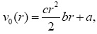 and so on.
Note that, despite of the specific form of L = αrmu(n) is known, there remains some arbitrariness in the choice of N, and even in the same L. What is more, in order to the method to work, in the limit p → 1, the sum αrmv(n) + N(v, p) must equal to A(v) (see (15)), because in this limit, the homotopy formulation (18) has to recover the original equation (16).
Again we propose that solution for (18) can be written as a power series of p (He 1998)
v = v0 + v1p1 + v2p2 +... (19)
When p → 1, it is expected to get an approximate solution for (14) in the form (He 1998; 1999;2000;2006;2008, Ganji et al; 2008;2009, Sharma and Methi 2011, Vazquez-Leal et al. 2012a; 2012b, Filobello-Nino et al. 2012a; 2012b)
v = v0 + v1 + v2 + v3 + ... (20)
Most of the examples that will be discussed are linear differential equations, because as it was mentioned, for these cases exist classical systematic methods of solution (see section 2) and it allow us compare and verify the performance of MNDHPM method.
6. - Application of MNDHPM to find power series solutions to differential equations.
The following examples show that MNDHPM method is particularly relevant for the case of non homogeneous differential equations with non polynomial coefficients, and non polynomial non homogeneous terms, regardless if the equation is linear or nonlinear. At the same time, we will emphasize the joining of HPM methods in the search for power series solutions.
Example 1. This example depicts the solution of an equation with polynomial coefficients,
y"-(1 + x)y = 0, y(0) = 1, y'(0) = 1. (21)
by using Standard HPM, MNDHPM, and power series method (Zill 2012).
Power Series.
Since the point x0 = 0, is an ordinary point of (21), a solution of the form

and establishing a recurrence relation

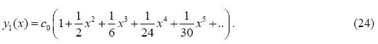
by iterating (23), we obtain the coefficients
c1 = 0, c2 = c0/2, c3 = c0/6, c4 = c0/24, c5 = c0/30,..
whose values are substituted into (22), obtaining a solution of the form
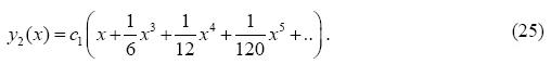
In the same way, iterating a second time, yields
c0 = 0, c2 = 0 c3 = c1/6, c4 = c1/12, c5 =c1/120,..
substituting these coefficients into (22) we obtain another solution
Note that for obtaining the n-th approximation, we need to calculate the n-th coefficient cn, of series development (22).
From (24) and (25), the general solution of (21), keeping to the fifth power of x, is expressed as

after applying the initial conditions y(0)=1 and y'(0)=1 to (26), we obtain the required solution
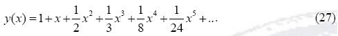
the process described is long for the most of practical applications.
Standard HPM
To find a power series solution by standard HPM method, we construct the following homotopy (see (7) and (8)).
(1 - p)( y" - y0'')+p( y" - (1+x) y) = 0 (28)
or
y"- y0"+p( y" - (1+x) y) = 0, (29)
where we have identified terms:
L = y''(x), (30)
N = -(1 + x) y( x). (31)
Substituting (9) into (29) and equating terms with identical powers of p, we obtain
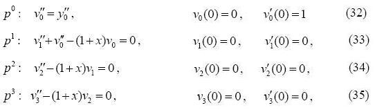 ...
...
To solve the above equations, we choose
v0(x) = 1 + x , (36)
as the first approximation for the solution of (21) that satisfies the initial conditions.
Solving the above equations, we obtain the following results
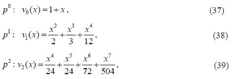
...
and so on.
Therefore, an approximate solution of (21) is obtained by substituting (37), (38), and (39) into (10), to obtain

As it can be seen, standard HPM requires only the second order approximation to generate up to the fifth power of x, with much less effort than the method of power series. In fact, it only requires to solve elementary integrals.
MNDHPM Method.
Following (11), we embed the parameter p as follows
(1 - p)( y'' - y0" )+p( y'' - p(1+x) y) = 0 (41)
or
y'' - y0''+p(y0'' - p(1+x)y) = 0, (42)
where, L and N are given by (30) and (31).
Substituting (19) into (42), and arranging coefficients with "p" powers we construct the following equations
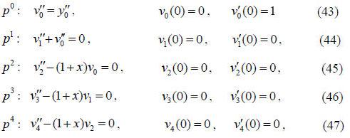
...
To solve the above equations, we choose
v0(x) = 1 + x , (48)
as the first approximation for the solution of (21) that satisfies the initial conditions.
Solving (43), (44), (45), (46) and (47) we obtain
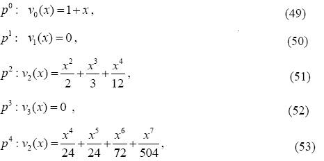
...
and so on.
Therefore, an approximate solution of (21) is obtained by substituting (49), (50), (51), (52) and (53) into (20), obtaining
As it can be seen, the embedding of p makes that terms of some orders of the approximation become zero, and are required iterations up to fourth order to achieve the fifth power of x. Although MNDHPM is simpler than the series methods in the search of series solutions, in the case of differential equations with polynomial coefficients is not better than standard HPM method.
Example 2. The following example compares in detail the methods HPM and MNDHPM.
y' + y = exp(x), y(0) = 0 (54)
By using an integrating factor (Zill 2012), equation (54) has the following exact analytical solution.
y = 1/2(exp( x) - exp(-x)) (55)
Standard HPM
To employ the standard HPM method, we construct the homotopy (see (7) and (8))
(1 - p)(y' - y0')+p(y '+y - exp(x)) = 0 (56)
or
y' - y0'+p(y0'+y - exp(x)) = 0, (57)
where we have identified terms:
L = y' (x), (58)
N = y(x) - exp( x). (59)
substituting (9) into (57), and equating terms with identical powers of p, we obtain
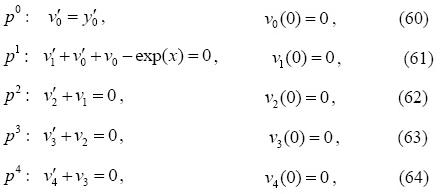
...
To solve the above equations, we choose
v0(x) = x , (65)
as the first approximation for the solution of (54) that satisfies the initial conditions.
Moreover, to obtain a solution in power series, we substitute
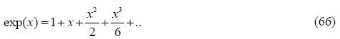
into (61), so that the solution of equations (60)-(64) is expressed as
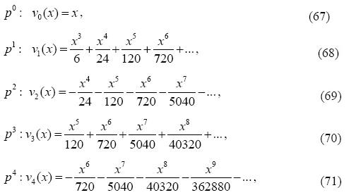
...
Therefore, an approximate solution for (54) is obtained by substituting (67)-(71) into (10), such that

after cancelling terms, (72) is reduced to
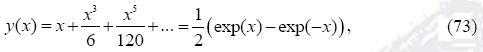
which is the solution shown in (55).
MNDHPM Method.
Following (18), we embed the parameter p as follows
(1 - p)(y' - y'0)+p(y+y - exp(px)) = 0 (74)
or
y' - y'0+p(y'0+y - exp(px)) = 0, (75)
where, L and N are given by (58) and (59).
Substituting (19) and
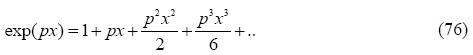
into (75), and equating terms having identical powers of p we obtain
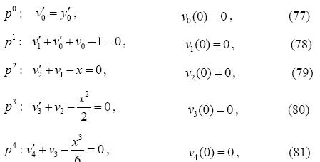
...
To solve the above equations, we choose
v0(x) = x, (82)
as the first approximation for the solution of (54) that satisfies the initial conditions.
Solving the above equations we obtain
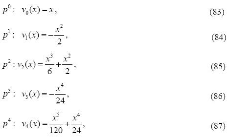
...
An approximate solution of (54) is obtained by substituting (83)-(87) into (20), so that

As can be seen, even in the case of simple equations such as (54), the presence of non polynomial terms, leads to the standard HPM method to introduce infinite series in the calculation of the various orders of approximation, this complicates the process of finding solutions. By contrast, such as it was shown with the above example, we will see that the MNDHPM eliminates these difficulties, at least for the case of equations with cosine variable coefficients and exponential inhomogeneous terms, although as it was mentioned, would be expected that it works also, for other functions N(v, p) and f (r, p), which can be expressed in terms of power series of p, and provides solutions of equations as (54), in a simple way, just by solving elementary integrals.
The following examples are resolved by using the MNDHPM method and then are compared with series method.
Example 3. This example, which presents a second order equation with non-polynomial variable coefficients, compares in detail HPM and MNDHPM, with power series method (Zill 2012).
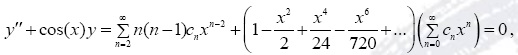
y" + cos(x)y = 0, y(0) = 1, y'(0) = 1. (88)
Power Series. Since the pointx0 = 0, is an ordinary point of (88), we seek a solution of the form
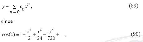
substituting (89) and (90) into (88), we obtain
after performing multiplications, and grouping terms having identical powers of p, we obtain
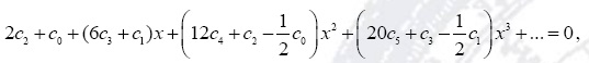
from this equation, the following system of equations is deduced
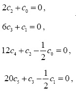
...
after solving the above equations for the coefficients, we obtain the general solution as follows
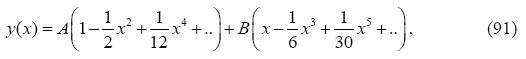
applying the initial conditions and, to (91), we obtain the required solution
MNDHPM Method
To find a power series solution by MNDHPM method, we construct the following homotopy (see (18)).
(1 - p)( y" - y0'') + P( y" + cos( px) y) = 0 (93)
or
y''- y''0+p( y0'' + cos( px) y) = 0, (94)
in homotopy (93) we have identified terms as follows:
L = y''(x), (95)
N = y(x)cos( x). (96)
substituting (19) and

into (94) and equating terms having identical powers of p we obtain
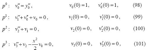
...
Let us select
v0(x) = 1+x, (102)
as an approximated solution of (88) that satisfies the initial conditions.
Solving the above equations we obtain the following results
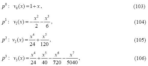
...
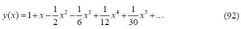
An approximate solution for (88) can be obtained, by substituting (103)-(106) into (20), such that we obtain again
We see that MNDHPM method requires only the third order approximation to generate up to the fifth power of x, with much less effort than the method of power series. As in the previous examples, it only requires solving elementary integrals.
Example 4. - Consider the following linear second order ordinary differential equation with no polynomial variable coefficients, which approximately describes the interaction of two nucleons (Arfken y Weber 1995).

with initial conditions, y(0)=0, y'(0)=a.
The above equation is the Schrödinger wave equation (Arfken y Weber 1995) for a meson potential , V = A exp(-x) / x, where A is a constant.
MNDHPM Method
To find a power series solution by HPM method with nonlinearities distribution, we construct a homotopy in the form
(1 - p)(xy'' - xy''0) + p(xy'' + yE'x - A' y exp(-px)) = 0, (108)
in the above homotopy we have identified the following terms:
L = xy" (x), (109)
N = [xE' - A' exp(-x)] y (x).(110)
Substituting (19) and the power series expansion
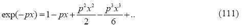
into (108), and equating the coefficients of terms with similar powers of p, we get
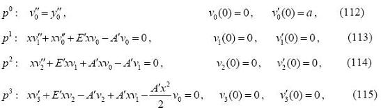
...
Let us take
v0(x) = ax, (116)
as an initial approximation for the solution of (107) that satisfies the initial conditions.
After solving the equations (112)-(115), we obtain
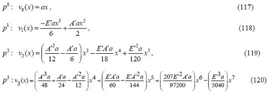
...
Thus the solution of (107) is obtained by substituting (117)-(120) into (20) to obtain
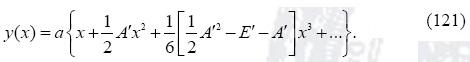
Since the point x0 = 0 is a regular singular point of (107), we can employ the Frobenius series method to obtain solution (121), by substituting (3) in (107) (Arfken y Weber 1995).
It should noted that the Frobenius method is even longer than the power series method described (see examples 1 and 3), and therefore, more than the MNDHPM.
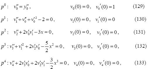
Example 5. - Consider the following nonlinear second order ordinary differential equation.
y" + y'2 - exp(2x) - exp(x) = 0, (122)
with initial conditions y(0) = 0, y'(0) = 1.
MNDHPM Method
To find a power series solution by modified HPM method with nonlinearities distributions, we construct a homotopy as follows
(1 - P)(y'' - y'0) + P[y'' + y'2 - exp(2px) - exp(px)] = 0, (123)
which can be grouped as
y'' - y0'' + P[y'' + y'2 - exp(2px) - exp(px)] = 0, (124)
where we have identified terms:
L = y''(x), (125)
N = [ y'2 (x) - exp(2x) - exp( x)]. (126)
Using the power series expansions
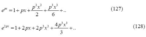
and substituting (19), (127) and (128) into (124), and then grouping coefficients with identical powers of p we obtain
...
To solve the above equations, we choose
v0(x) = x (134)
as an initial approximation for the solution of (122) that satisfies the initial conditions, thus
p0: v0( x) = x, (135)
p1: v1(x) = x2/2, (136)
p2: v2( x) = x3/6, (137)
p3: v3(x) = x4/24, (138)
p4; v4( x) = x5/120, (139)
...
The substitution of (135)-(139) into (20), shows that the resulting series can be expressed in a closed form as
y(x) = 1 + x + x2/2 + x3/6 + x4/24 + x5/120 +...-1 = ex-1, (140)
To emphasize the usefulness of HPM methods in the search for solutions of differential equations in terms of power series, the following equations with polynomial coefficients are solved by using the standard HPM method.
Example 6. - Consider the linear first order ordinary differential equation.
y' + 2 xy = 0, (141)
with initial condition y(0) = 1.
We construct the following homotopy
(1 - p)(y ' - y0')+p(y'+2xy) = 0, (142)
or
y' - y'0+p(y'0+2xy) = 0, (143)
Substituting (9) into (143) and proceeding as in the previous examples, is obtained a resulting series which can be expressed in a closed form as
y(x) = 1 - x2 + x4/2 - x6/6 +... = exp(- x2). (144)
Since the point x0 = 0 is an ordinary point of (141), the Power Series Method could be employed to obtain solution (144), by substituting (2) in (141) (Zill 2012).
Example 7. – Consider Hermite,s differential equation which has applications in physical sciences (Arfken y Weber 1995).
y" - 2xy' + 2αy = 0, where α is a constant, (145)
with initial conditions y(0) = a, y'(0) = 0.
Following the above procedure, it is obtained the solution
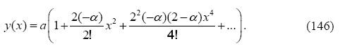
The point x0 = 0 is an ordinary point of (145), and therefore it can be employed the power series method in order to obtain solution (146), by substituting (2) in (145) (Arfken y Weber 1995).
7. – Discussion
7.1. - MNDHPM and Standard HPM Methods.
This paper proposes the MNDHPM method, as a tool to find power series solutions of both linear and nonlinear ordinary differential equations with initial values. From the examples explained, we found that MNDHPM and standard HPM provide the same results with similar complexity for the case of polynomial coefficients, and/or polynomial nonhomogeneous term (see example 1), where the use of standard HPM is adequate. On the other hand, MNDHPM method shows better results when those functions are non polynomial, such as exponentials used in the examples. Example 2 showed that application of standard HPM method to equations with non polynomial nonhomogeneous terms, although is not complicated, infinite series may occur at the different iterations, complicating the process of solution, in special for the case of more complicated equations.
In Example 5, the MNDHPM method was employed to find a power series solution of a nonlinear ordinary second-order differential equation. Unlike previous reports in the literature that apply the standardized approach for HPM solutions of nonlinear differential equations using power series (Ganji 2009, Hossein 2011) this work demonstrates the utility of the proposed modified HPM method with nonlinearities distribution, especially in equations which include non polynomial coefficients and/or non polynomial nonhomogeneous terms, as the cosine and exponentials functions used in examples, showing a better performance.
The main reason is that MNDHPM distributes the contributions of coefficient functions along the iterations in the differential equations for the successive parameter powers p: p: p0,p1,p2,..., that allows to MNDHPM method being simpler at the different stages of iterations. Moreover, is relevant that those results are valid for both linear and nonlinear ordinary differential equations. In fact, the use of the modified HPM method with nonlinearities distribution, for the case of differential equations with non-polynomial coefficients and/or non polynomial nonhomogeneous terms is considered as the main contribution of this work.
7.2. - HPM Methods and Solutions by Series.
As it was seen, the solutions of linear differential equations obtained by using HPM methods and the method of power series were the same for our examples. In particular examples 1 and 3 showed and compared the use of HPM and MNDHPM with series method and it was emphasized the effort invested in each case. The solution for an initial value problem, employing the classical methods of series based in (2) and (3), turns out to be many times long and requires initially finding a general solution for the equation before employing the initial conditions to find the solution that is needed. Another problem that arises in the case of regular singular points, is that frequently the Frobenius method does not directly provide two linearly independent solutions, only one, and a second solution needs to be found, which implies solve integrals that usually contains infinite series (Zill 2012), and that causes the use of these methods become complicated for practical applications. This contrasts with the results obtained by HPM methods, which only require uncomplicated integrals to provide the solution. This occurs because since the beginning, the initial approximation function is chosen as simple as possible, besides satisfying initial conditions. An important contribution of this work was emphasize the usefulness of HPM methods in the systematically search for solutions to differential equations in terms of power series.
Respect to convergence of solutions obtained by standard HPM method, those issues are addressed in (He 1999; 2000, Biazar y Aminikhan 2009a, Biazar y Ghazvini 2009b) while the ones of MNDHPM method, can be discussed in a similar way as in (Vazquez Leal et al. 2012a).
8. – Conclusions
The solution methods for linear differential equations of variable coefficients are based on classical methods for infinite series, mentioned in section 2.
Nevertheless, the solution to initial conditions problems, by employing these methods, for some cases it requires a great computational effort. To overcome this shortcoming, this paper explored the possibility to employ MNDHPM in order to solve linear and nonlinear ordinary differential equations, with initial conditions. Despite the fact that MNDHPM does not offer clear advantages over standard HPM for the case of polynomial coefficients, its performance is better for some equations with no polynomial coefficients and/or no polynomial nonhomogeneous terms as the cases study of this work.
It is worth mentioning that the Homotopy Perturbation Methods studied here, are capable of reducing the computational work as compared to the classical methods based on (2) and (3), because these techniques only require of simple integrals to obtain the same results. It is relevant that the above considerations are valid also for the nonlinear differential equations of example 5 and perhaps for other similar cases.
References:
Agida M, Kumar AS. (2010). A Boubaker Polynomials Expansion Scheme solution to random Love equation in the case of a rational kernel. El. J. Theor. Phys, 7 (2010) 319-326. [ Links ]
Aminikha, Hossein. (2011) Analytical Approximation to the Solution of Nonlinear Blasius Viscous Flow Equation by LTNHPM. International Scholarly Research Network ISRN Mathematical Analysis, Volume 2012, Article ID 957473, 10 pages. [ Links ]
Arfken, George y Hans Weber (1995). Mathematical Methods for Physicists, Fourth Edition. Academic Press, Inc. [ Links ]
Biazar, J.y H. Aminikha (2009a). Study of convergence of homotopy perturbation method for systems of partial differential equations. Computers and Mathematics with Applications, Vol. 58, No. 11-12, (2221-2230). [ Links ]
Biazar, J. y H. Ghazvini (2009b). Convergence of the homotopy perturbation method for partial differential equations. Nonlinear Analysis: Real World Applications, Vol. 10, No 5, (2633-2640). [ Links ]
Chowdhury, SH. (2011). A comparison between the modified homotopy perturbation method and a decomposition method for solving nonlinear heat transfer equations, Journal of Applied Sciences, 11: 1416-1420. [ Links ]
Evans DJ, Raslan. KR (2005). The Tanh function method for solving some important nonlinear partial differential. Int. J. Computat. Math., 82: 897-905. [ Links ]
Filobello-Nino, U, H. Vazquez-Leal, R. Castaneda-Sheissa, A. Yildirim, L. Hernandez-Martinez et al (2012a). An approximate solution of Blasius equation by using HPM method. Asian J. Math. Stat., 5: 50-59. [ Links ]
Filobello-Nino, U, H. Vazquez-Leal, Y. Khan, A. Yildirim, D. Pereyra-Diaz et al (2012b). HPM applied to solve nonlinear circuits: A study case. Applied Math. Sci., 4331 - 4344.
Filobello-Nino, U, H. Vazquez-Leal, Y. Khan, A. Yildirim, D, VM. Jimenez-Fernandez et al (2012c). Perturbation method and Laplace-Pade approximation to solve nonlinear problems. Miskolc Mathematical Notes. (In Press).
Ganji, DD, H. Babazadeh, F. MM. Noori, Pirouz, M. Janipour (2009). An application of homotopy perturbation method for non linear blasius equation to boundary layer flow over a flat plate. Int. J. Nonlinear Sci. Vol.7, No.4: 309-404. [ Links ]
Ganji, DD, H. Mirgolbabaei, M. Miansari (2008). Application of homotopy perturbation method to solve linear and non-linear systems of ordinary differential equations and differential equation of order three. Journal of Applied Sciences, 8: 1256-1261. [ Links ]
Ghanouchi, J, H. Labiadh, K. Boubaker (2008). An attempt to solve the heat transfert equation in a model of pyrolysis spray using 4q-order m-Boubaker polynomials Intl. J. of Heat and Technology, 26: 49-53. [ Links ]
He, JH. (1998). A coupling method of a homotopy technique and a perturbation technique for nonlinear problems. Int. J. Non-Linear Mech., 351: 37-43. [ Links ]
He, JH. (1999). Homotopy perturbation technique. Comput. Methods Applied Mech. Eng., 178: 257-262. [ Links ]
He, JH. (2000). A coupling method of a homotopy and a perturbation technique for nonlinear problems. International Journal of Nonlinear Mechanics, 35(1): 37-43. [ Links ]
He, JH (2006). Homotopy perturbation method for solving boundary value problems. Physics Letters A, 350(1-2): 87-88. [ Links ]
He, JH. (2008). Recent Development of the Homotopy Perturbation Method. Topological Methods in Nonlinear Analysis, 31.2: 205-209. [ Links ]
Kazemnia M, SA. Zahedi, M. Vaezi, N. Tolou (2008). Assessment of modified variational iteration method in BVPs high-order differential equations. Journal of Applied Sciences, 8: 4192-4197. [ Links ]
Khan, Y y Q. Wu (2011). Homotopy perturbation transform method for nonlinear equations using He's polynomials. Computers and Mathematics with Applications, Vol. 61, No. 8: 1963-1967. [ Links ]
Kooch, A y M. Abadyan (2011). Evaluating the ability of modified Adomian decomposition method to simulate the instability of freestanding carbon nanotube: comparison with conventional decomposition method. Journal of Applied Sciences, 11: 3421-3428. [ Links ]
Kooch, A y M. Abadyan (2012). Efficiency of modified Adomian decomposition for simulating the instability of nano-electromechanical switches: comparison with the conventional decomposition method. Trends in Applied Sciences Research, 7: 57-67. [ Links ]
Mahmoudi, JN. Tolou, I. Khatami, A. Barari, DD. Ganji (2008). Explicit solution of nonlinear ZK-BBM wave equation using Exp-function method. Journal of Applied Sciences, 8: 358-363. [ Links ]
Mirgolbabaei, H y DD Ganji (2009). Application of homotopy perturbation method to solve combined Korteweg de Vries-Modified Korteweg de Vries equation. Journal of Applied Sciences, 9: 3587-3592. [ Links ]
Noorzad R, AT Poor, M. Omidvar (2008). Variational iteration method and homotopy-perturbation method for solving Burgers equation in fluid dynamics. Journal of Applied Sciences, 8: 369-373. [ Links ]
Patel, T y MN. Mehta, VH. Pradhan (2012). The numerical solution of Burger's equation arising into the irradiation of tumour tissue in biological diffusing system by homotopy analysis method. Asian Journal of Applied Sciences, 5: 60-66. [ Links ]
Saravi, M, M. Hermann, D. Kaiser (2013). Solution of Bratu's equation by He's Variational Iteration method. American Journal of computational and applied mathematics, 3(1):46-48. [ Links ]
Sharma, PR y G Methi (2011). Applications of homotopy perturbation method to partial differential equations. Asian Journal of Mathematics & Statistics, 4: 140-150. [ Links ]
Tolou, N J, M. Mahmoudi, I. Ghasemi, A. Khatami, Barari, DD. Ganji (2008). On the non-linear deformation of elastic beams in an analytic solution. Asian Journal of Scientific Research, 1: 437-443. [ Links ]
Vanani, SK, S. Heidari, M. Avaji (2011). A low-cost numerical algorithm for the solution of nonlinear delay boundary equations. Journal of Applied Sciences, 11: 3504-3509. [ Links ]
Vazquez-Leal, H, U. Filobello-Nino, R. Castaneda-Sheissa, L. Hernandez-Martinez, A. Sarmiento-Reyes (2012a). Modified HPMs inspired by homotopy continuation methods. Mathematical Problems in Engineering. Vol. 2012. [ Links ]
Vazquez-Leal, H, R. Castaneda-Sheissa, U. Filobello-Nino, A. Sarmiento-Reyes, J. Sánchez-Orea (2012b). High accurate simple approximation of normal distribution related integrals. Mathematical Problems in Engineering, Vol. 2012. [ Links ]
Zill Dennis (2012). A First Course in Differential Equations with Modeling Applications, 0th Edition. Brooks /Cole Cengage Learning. [ Links ]

