Ciencias naturales e ingenierías

 

Spread in time of some bacterial infectious diseases: a mathematical model

 

Propagación temporal de algunas enfermedades bacterianas: un modelo matemático

 

R. Cipolatti¹, J. López Gondar^{2, 3} y E. Siqueira¹

 

¹ Departamento de Métodos Matemáticos, Universidad Federal de Río de Janeiro, Brasil.

² Departamento de Matemática Aplicada, Universidad Federal de Río de Janeiro, Brasil.

³ Instituto de Matemática, Universidad Federal de Río de Janeiro, Brasil.

 

Instituto de Matemática, Universidad Federal de Río de Janeiro, C.P. 68530, Rio de Janeiro, Brasil. E-mail: gondarj@yahoo.es

 

Recepción: 26-04-2012 
Aceptación: 15-05-2012

 

Abstract

We introduce a new theoretical model to describe the dynamics of transmission for a certain class of bacterial infectious diseases. The propagation mechanism considered is the one concerning direct personal contact. Immunity factors, if present, will be ignored, but in our calculations is included the existence of an incubation period for the contagious infection. The effects of public health campaigns on the spread of the disease are also considered and the inclusion of a certain parameter ε to measure the efficiency of such attempts is proposed.

Key words: Infectious diseases, nonlinear delay equations, asymptotic behavior.

 

Resumen

Introducimos aquí un nuevo modelo teórico para describir la dinámica de transmisión a que responden algunas enfermedades infecciosas bacterianas. El mecanismo de propagación considerado es el de contacto personal directo. La presencia de factores de inmunidad es ignorada, pero el modelo incorpora la existencia de un período de incubación para la enfermedad. Los posibles efectos de campañas educativas de salud pública, orientadas a controlar la propagación, son incluidos y se introduce un cierto parámetro ε para cuantificar la eficiencia de ese tipo de recurso.

Palabras clave: enfermedades infecciosas, ecuaciones no lineales de retraso, comportamiento asintónico.

 

1. Introduction

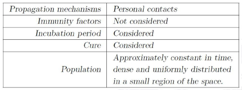
Infectious diseases represent not only a kind of social problem but also a source of economically harmful effects. Expenses with medical assistance as well as with prophylactic actions are usually the best-known negative effects, although the loss of productivity equally plays an important role. Because of these and other reasons, a lot of papers and books have been devoted during the last decades to obtain and describe mathematical models capable to reproduce, in a relatively reliable form, the dynamics of transmission for different types of contagious diseases (see, for instance [6,8,10,12,13,14,15,16,17] and the references therein). From the historical point of view it is fair to emphasize at this point that the pioneer in the formulation and application of deterministic models to the study of contagious diseases, was the Dutch-Swiss mathematician Daniel Bernoulli. In 1760, he developed a mathematical method to investigate the effectiveness of variolation (also referred to as inoculation) against smallpox [1]. Smallpox is an infectious disease, unique to humans, of viral origin.

In this paper we won't deal with viral diseases, but with a certain kind of infectious bacterial illness like pneumonia or tuberculosis, for instance, subjected to an adequate outpatient treatment. Such kinds of diseases are transmitted only by direct contact (without the participation of any kind of vector) and, in order to construct our simplified model, we shall start considering that the sample resembles a geographically homogeneous and dense population distribution. To ensure that all potential physical contacts among individuals be equally likely to occur, we assume that the population is concentrated in a small enough spatial region. We also assume that there exists a maximum time interval T₀ (the same for all infected individuals) during which an individual can withstand without medical assistance being a carrier of the infection. After this time, any recovery attempt is doomed to failure and, in general, the patient dies. For shorter times, however, the cure, following a proper treatment, is guaranteed. It is just for this reason that we shall consider that all the infectious individuals will be subjected to an adequate medical treatment, at most up to T₀. This maximal time can be reduced, in the best of the cases, to the value T₁ < T₀ by means of adopting more efficient health politics: for example, through campaigns to alert the population, with the objective to seek for medical help as soon as the first symptoms of the disease appear.

The infection process begins with a contact between a susceptible individual and an infectious one. From this moment, the first individual is contaminated (infected, but not yet infectious) remaining in such a state during a time t₀ < T₁ after which he becomes a disease transmission agent. Such an interval is called the incubation period [1]. Under these considerations and including some additional hypothesis, we construct in Section 2 a mathematical model to study the dynamics of transmission in the presence of proper medical assistance. In Section 3, a mathematical analysis of the system of integral equations, which represents the model previously obtained, is performed. To conclude, in Section 4 an alternative to reduce endemic levels is proposed and some conditions under which the disease can be definitively eliminated from the population (here considered as a closed system by hypothesis), are described. Numerical results and final comments are also included in this section.

 

2. Developing the mathematical model

The main hypothesis that we shall use here can be summarized as follows.

On the other hand, our universe is constituted by three different co-existing classes:

a) the class S of susceptible people (neither infected nor infectious),

b) the class I of infectious or infective individuals (those capable to transmit the infection) and

c) the class C of contaminated individuals, which are infected but can't transmit the infection yet.

Using the total size N of closed host population as a normalization factor, one can associate to the classes declared above the probabilities S₀(t), I₀(t) and C₀(t), respectively; where

 

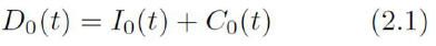
represents the probability to find an infected individual in the population and So(t) + Do(t) = 1.

Let us also introduce a function of two variables P₀(t, τ ), P₀ : Λ → [0, 1], where

which represents the probability that someone infected at τ remains infected at t. This function is I supposed to have the following heuristic properties:

 

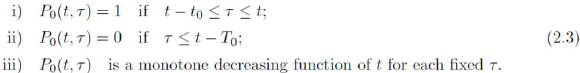
Remark 2.1: In most situations we can consider the probability P0 in the form

P₀(t, τ ) = φ₀(t - τ ), where φ₀ : [0, + ∞) → R satisfies

 An adequate contact-propagation equation can be written as [2,3]:

where g(τ) is the rate of the infection process (number of new infected individuals per unit time, at the instant τ , divided by N ). Notice, from Eq. (2.5), that if one wants to describe the probability to find an infected individual at time t, the integration should be performed only along the interval [t - T₀, t], just because of the existence of a maximum recovery time T₀. Taking into account that among all the possible contacts the only ones that could transmit the infection are those involving infective and susceptible individuals, the probability of an infectious contact to occur is I₀(t)S₀(t) = I₀(t)[1 - D₀(t)]. Then, denoting by α(τ) the capacity to infect, which we shall define in this case as the probability per unit time that a susceptible in contact with an infectious becomes infected, we obtain g(τ ) = α(τ)I₀(τ )[1 - D₀(τ )], where α(τ) is a positive function on [-T₀, + ∞).

Under these considerations, the contact-propagation equation Eq. (2.5) adopts the form

 

On the other hand, taking into account that any individual contaminated at t must remain in such a state only up to t + t₀ (probability 1) before becoming infectious, we have

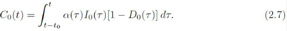
The equations (2.1), (2.6) and (2.7) now should be written as the system which describes de dynamics of the disease, namely

Notice that if t₀ = 0, D₀(t) = I₀(t) and the system (2.8) reduces to an equation for D₀(t), which coincides with the one proposed by Cooke-Yorke [5] in their model for gonorrhea. Furthermore, it is important to point out that the infectious individuals can also contaminate susceptible ones even when they do not stay together at the same place and at the same time (a situation not considered in the present model). This is possible if the bacteria involved can remain active in the environment during certain time interval large enough. This situation could be identified as an indirect contact and, to describe it, we need to introduce new time delays in the integral equations, as it has been done in [4,9]

Observe that to obtain meaningful solutions for the system (2.8), it is necessary to guarantee that

As the above inequalities imply that

Haga clic para agrandar

 

it is easy to see that

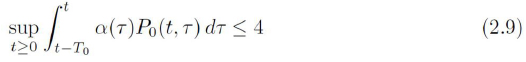
is a sufficient condition for solutions which actually represent probabilities.

 

3. Mathematical Analysis of the Model

In this section we present some results on the dynamic of the solutions for the system (2.8). Before proceeding with the analysis, it is convenient to write this system as a vector integral I equation. Let χ : ℝ → ℝ be the characteristic function of the interval [0, t₀)], i.e.,

Then, omitting for the moment the subscripts to simplify the notation, the equation (2.7) can be written as

Moreover, since C = D - I , we have

 

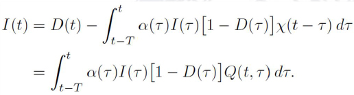
where Q(t, τ ): = P (t, τ ) - χ (t - τ). So, we have the system

 

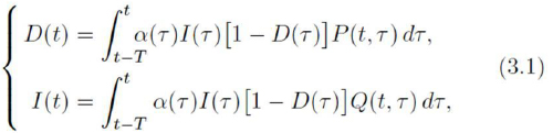
Now, we are in position to write (3.1) as a vector equation. Let us consider the vector functions

 

With this notation, the system (3.1) can be written as

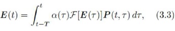
where 𝓕 : ℝ²→ℝ is defined by 𝓕[(x,y)]:= y(1—x).

Let L^∞(-T, + ∞) be the space of Lebesgue measurable and bounded functions on [-T, + ∞) endowed with the usual norm k k_L^∞, namely,

We denote 𝕍 = L^∞(T, + ∞) x L^∞(T, +∞), which is a Banach space for the norm ∥E∥v= ess sup {∥E(τ)∥; τ ≥ -T}, where ∥ ∥ is the usual infinite-norm of ℝ², i.e, ∥u∥= max{∣x∣,∣y∣}, for all for u = (x,y) ∈ ℝ².

 

In view of the model we have in mind, it is natural to restrict our analysis to the solutions E ∈ V, E (t) = (D(t), I (t)) such that D(t), I (t) ∈ [0, 1] for all t ≥ -T . Moreover, since D(t) ≥ I (t), we can consider the following set of "admissible functions".

 

It is clear that A is a bounded and closed subset of V

In what follows, we consider the set Λ defined by (2.2) and the vector function P : Λ → [0, 1] x [0, 1], P = (P, Q) as defined in (3.2). We also assume that α is a positive and locally Lebesgue integrable function in (-T, + ∞)

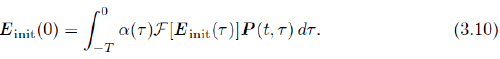
Definition: Let E _init ∈ V. We will say that a function E ∈ V is an admissible solution of Eq. (3.3) generated by E _init if E ∈ A and

The following propositions establish uniqueness and existence of solutions for the Eq. (3.3). Their proofs are based on standard methods involving Gronwall inequality and Banach Fixed Point Theorem and will be omitted.

Proposition 3.1: Let α satisfying (3.5) and E _init ∈ V. If E₁ and E₂ are admissible solutions of Eq. (3.3) generated by E _init, then E₁(t) = E₂(t) for all t > 0.

For the existence of solutions, we consider the functions r_D (t) and r_I (t) defined by

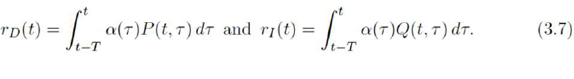
In the particular case where α is constant and P (t, τ ) = φ(t - τ ), these two functions are constant with values given by

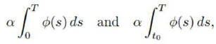
respectively.

Proposition 3.2: Assume that α satisfies (3.5) and r_D (t) ≤ 4 for all t ≥ 0. For each E _init∈ A, there exists E , a unique admissible solution of Eq. (3.3) generated by E _init.

Remark 3.3: To prove Proposition 3.2 we consider the set

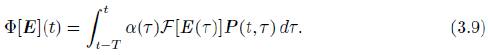
which is a closed and bounded subset of V and we apply Banach's Fixed Point Theorem to the operator Φ : A (E _init) → A (E _init) defined as Φ [E](t) = E _init(t) almost everywhere in [- T , 0] and, for t > 0,

By this approach, the condition r_D (t) ≤ 4 becomes necessary because, otherwise, the set A(E _init) defined in (3.8) may not be an invariant set for the operator Φ. Indeed, consider for instance E (t) = (c₁, c₂ ) for all t ≥ - T , where 0 ≤ c₂ ≤ c₁ ≤ 1. Then,

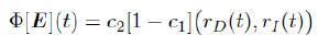
and we have Φ[E ] ∉ A if we choose c₁ and c₂ such that c₂ (1 - c₁ ) > 1/4.

Remark 3.4: As an immediate consequence of the absolute continuity of the Lebesgue integral, it follows that E is continuous on the interval ]0, + ∞ [. In order to assure its continuity in [- T , + ∞ [, it is sufficient to assume that E _init is continuous on [- T , 0] and satisfies the following compatibility condition:

 

• Asymptotic Behavior:

In this subsection we shall study the asymptotic behavior of the solutions assuming that r_I (t) ≤ 1 for t large enough.

Theorem 3.5: (a) Assume that a satisfies (3.5) and r_D (t) ≤ 4 for all t ≥ 0. Let E = (D, I) be the unique admissible solution of Eq. (3.3) generated by E_init ∈ A. If

 

then there exist C, M, L > 0 such that

(b) Moreover, if α is constant, P (t, τ ) = φ(t − τ ) and they are such that

then

 

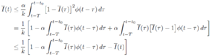
Proof: (a) We assume that the condition (3.11) holds. Then, there exist 0 ≤ ρ < 1 and M > 0 such that r_I (t) ≤ ρ for all t ≥ M . If we denote E (t) = (D(t)), we have

Haga clic para agrandar

 

If we define φ(s): = sup{Ī(τ); τ ∈ [s, + ∞)}, then we have for t ≥ M,

Now, by noting that Φ(s) is a decreasing function, it follows that sup{Φ(s) ; s ≥ t} = Φ(t). Hence, taking the supremum for t ≥ s in (3.15), we obtain

By considering successively s = M + T , M + 2T , . . ., we have

Therefore, for t > M and k ∈ N such that t ∈ [M + kT , M + (k + 1)T ), we have

where c: = e^{−(M +T )L} Φ(M ) and L: = − ln ρ/T . Moreover,

Haga clic para agrandar

and we obtain kE (t)k = D(t) ≤ C e^-Lt , ∀ t ≥ M , where C : = 4ce^LT . Being so, the proof of part (a) is complete.

(b) Now, we assume that α is constant, P (t, τ) = φ(t - τ ) and that they are such that (3.13) holds. We notice, first of all, that I (τ ) ≤ D(τ) implies

In particular, since 0 ≤ I (t) ≤ 1, we have the following inequalities that will be useful in the sequel:

 

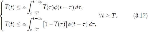
In order to obtain (3.14), we shall prove by mathematical induction the following inequality

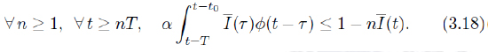
Step 1 : Let n = 1. From (3.13) and (3.17)₂, it follows that

from which we deduce that

Step 2: Now, we assume that (3.18) holds for n = k. Then, from (3.17)₁, we have

so kI(t) ≤ 1 - I(t) for all t ≥ kT. Substituting in Eq. (3.16) and remembering that I(τ) ≤ D(τ), we have for t ≥ (k + 1)T,

Haga clic para agrandar

 

and conclude that (3.18) holds for n = k + 1.

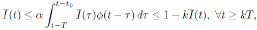
Notice that (3.18) and (3.17)₁ implies that I (t) ≤ (n + 1)^-1for all t ≥ nT . Hence, for nT ≤ t ≤ (n + 1)T , we have

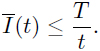
On the other hand, since 0 ≤ D(t ) ≤ 1, we obtain for t > T ,

Haga clic para agrandar

and the proof is complete.

 

• Stationary solutions:

As we will see now, under certain conditions, the system (3.1) admits nontrivial stationary solutions, i.e., nonzero solutions that do not depend on time. Notice that the trivial vector E (t) = (0, 0) is always a solution. Moreover, if α(t) = α > 0 is constant and P (t, τ ) = φ(t - τ ), where φ satisfies (2.4), then, assuming that E (t) = (D_∞, 1_∞) is a constant solution, we have from (3.1),

 

So, for I_∞ = 0, we get from the second equation of (3.19),

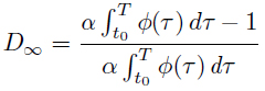
and since

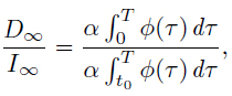
we get

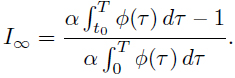
It is important to point out that if ρ := α φ(τ) dτ < 1, the above stationary solutions are inadmissible for the problem we are considering, i.e., (D_∞ , I_∞) ∉ A.

Nevertheless, in this case, any admissible solution converges to zero exponentially, as proved in Theorem 3.5. Moreover, I_∞ = D_∞ = 0 if ρ = 1 and, again, Theorem 3.5 assures that any admissible solution converges to zero. Besides, if ρ > 1, numerical u experiments lead us to expect that the following global asymptotic behavior for any solution E (t) holds:

 

4. Reduction of endemic levels, numerical results and conclusions

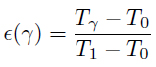
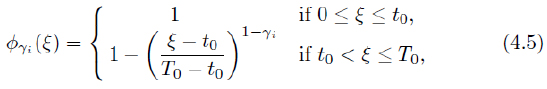
The probability function P₀ (t, τ) described in Eq. (2.3) depends, among other factors, on the time between the instant at which infectious individuals begin to feel the symptoms of the disease and the one when they will seek and obtain medical assistance. This individualized response time, as noted in Section 1, can not be greater than T₀ because, if so, the patient will die. On the other hand, the response time has also a lower bound t₀ (the incubation time). Let us now suppose that we develop an intensive educational campaign directing people to seek for medical care as soon as they perceive the symptoms of the disease. If the affected people respond favorably to that effort, in a greater or lesser extent, a new probability P_ϒ : Λ → R, instead of P₀ (t, τ ), must be considered. Like Eq. (2.3), we assume that

Haga clic para agrandar 

where T₁ ≤ T_ϒ ≤ T₀ is a new maximum recovery time for each case. Moreover, new probabilities to find contaminated, infective and susceptible individuals must be introduced and we shall denote them by C_ϒ(t), I_ϒ (t) and S_ϒ(t), respectively; being D_ϒ(t) = I_ϒ(t) + C_ϒ(t) and S_ϒ(t) + D_ϒ (t) = 1. Being so, equations (2.8) now should be written as

Haga clic para agrandar

 

In fact, the system (4.2) can be regarded as a family of systems depending on the parameter _{ϒ ∈} [0, 1], where _ϒ = 0 corresponds to the case in which no public health campaign is carried out.

It is obvious that all the results obtained in Section 3 also hold in this situation. Notice that under the hypothesis mentioned above, the value of the integral r_I (t) introduced in (3.7), should be smaller for P = P_ϒ than for P = P₀ . This fact allows to reduce the "standard" endemic levels of the disease in the affected population or, even, it could contribute to eliminate the illness itself, as we shall see below.

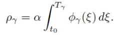
At this point, to characterize in a certain sense the efficiency of the efforts invested in order to reduce the number of people infected, it would be reasonably to define the function Q(_ϒ) as

where

 

and T₀, T₁ as already introduced in Section 1.

Notice that if α is constant and P_ϒ (t, τ) = φ_ϒ (t - τ), we have

In particular, if Φ : (0, 1) - [0, 1] is a decreasing function and if we define

then (4.3) reduces to

and we obtain T_ϒ = T₀ + Q(_ϒ) T₁ - T₀ .

It would be useful to point out that this last formula works only in the case T_ϒ< T₀ (? > 0), while Eq. (4.3) also includes the case T_ϒ= T₀ for all ? , at which, in spite of the efforts developed, some people insist to seek for medical assistance only when they are very sick.

 

• Numerical simulations:

In order to illustrate the time evolution behavior of the infection process governed by our model, we shall perform some numerical simulations. As it can be seen from the system (4.2), computational calculations in this direction demand a previous knowledge of part of the history of the illness evolution: more specifically, the history corresponding to the interval - T₀ ≤ t ≤ 0. Taking into account that our present purpose is only to exemplify and not to reproduce real situations, we may look at arbitrary functions to characterize I_ϒ(τ) and D_ϒ(τ) in the above mentioned interval. Furthermore, the capacity of infection α will be considered as a constant.

For the numeric simulations, we consider T₀ = 10, T₁ = 5, t₀ = 4 and E _init(t) = (0.5, 0.4). In each of the Figs. 1-4, (Figs. 2, 3, 5, 6) corresponding to the values α = 0.5, 0.7, 1.0, and 1.3, respectively, we present the graphics of D_ϒi (t), (i = 1, 2, 3), for _ϒ1 = 0, _ϒ2 = 0.4, _ϒ3 = 0.8, T_ϒi= T₀ + _ϒi (T₁ - T₀ ) and P_ϒi (t, τ ) = φ_ϒi(t - τ ), where

 

 

Conclusions:

In this paper we develop a model constituted by a system of delay integral equations, in order to perform a systematic study of the spread in time of some infectious bacterial diseases. It is supposed that the type of illness we deal with in the present article has a finite time to be successfully treated but also that, if this time is exhausted and the patient continues without medical assistance, he will unavoidably die. Other fundamental as well as simplifying working hypothesis are also listed in Sections 1 and 2. As a first attempt in understanding the dynamics of transmission, the possible presence of immunity factors was ignored (compatible with diseases like pneumonia and tuberculosis rather than with diphtheria and whooping cough, for example, for which there already exist vaccines), but the presence of a certain latent period for the illness is included, resembling a more realistic situation. Once the model was developed, we carried out the analysis concerning the assymptotic bahavior of solutions and we present numerical simulations to illustrate the trends of the spread of the disease over time. Some important properties were found and the ones we consider more relevant are summarized below.

An interesting feature of this model is that it is possible to extinguish the infection process and, consequently, the disease itself, as can be seen in the figures above. Indeed, from Theorem 3.5 one concludes that all solutions of Eq. (3.3) decay to zero if ρ_ϒ ≤ 1 (exponentially if ρ_ϒ< 1). Hence, ρ₁ < 1 is a sufficient condition for the existence of some 0 ≤ _ϒ < 1 which ensures the abortion of the transmission process and with it the extinction of the disease. Furthermore, one also intuit from these figures that when there are no conditions to extinguish the disease, the functions D(t) (I (t)) tends to a constant value characterizing an endemic situation. The introduction in this work of the parameter Q, which can be obtained experimentally by indirect measurements, allows estimating an index connected with the efficiency of the efforts displayed to eliminate the disease or, at least, to reduce the corresponding endemic levels.

Studies considering space-time spreading are also now in progress and will be published elsewhere.

 

Acknowledgements

The authors would like to acknowledge Alexandre Siqueira (Fundação Oswaldo Cruz) for useful discussions.

 

References

[1] Bailey, N.J.T.: The mathematical theory of infectious diseases and its applications; Griffin, London, 1975.         [ Links ]

[2] Bellmann, R., Cooke, K.L.: Differential-difference equations; Math. in Sciences and Engineering, Academic Press, 1963.         [ Links ]

[3] Capasso, V.: Mathematical structure of epidemic systems ; Springer-Verlag, 1993.         [ Links ] [4] Cipolatti, R., Lopez Gondar, J.: Dynamics of a virtual virus infection process in volving a spatial distribution of interacting computers ; Applicable Analysis: An International Journal, 1563-504X, Volume 84, Issue 1, (2005,) pp. 49-65.         [ Links ]

[5] Cooke, K.L., Yorke, J.A.: Some equations modelling growth processes and gonorrhea epidemics ; Mathematical Biosciences, #16 (1973), pp. 75-101.         [ Links ]

[6] Cui, C., Sun, Y., Zhu, H.: The impact of media on the control of infectious diseases; Journal of Dynamics and Differential Equations, Vol. 20, No. 1, (2008), pp. 31-53.         [ Links ]

[7] Driver, R.D.: Ordinary and delay differential equations ; Applied Mathematical Sciences #20, Springer-Verlag, 1977.         [ Links ]

[8] Diekmann, O., Heesterbeek, J.A.P.: Mathematical epidemiology of infectious diseases. Model building, analysis and interpretation ; John Wiley & Sons, Ltd., Chischester, 2000.         [ Links ]

[9] Lopez Gondar, J., Cipolatti, R.: A mathematical model for virus infectious in a system of interacting computers; Comp. Appl. Math., Vol. 22, No. 2, (2003), 209-231.         [ Links ]

[10] Ghosh, M., Chandra, P., Sinha, P., Shukla, J.B.: Modelling the spread of bacterial infectious disease with environmental effect in a logistically growing human population; Nonlinear Anaysis: Real World Applications, No. 7, (2006), 341-363.         [ Links ]

[11] Hale, J.: Theory of functional differential equations ; Applied Mathematical Sciences #3, Springer-Verlag, 1977.         [ Links ]

[12] Hethcode, H.D., Tudor, D.W.: Integral equation models for endemic infectious diseases ; Journal of Mathematical Biology, No. 9, (1980), 37-47.         [ Links ]

[13] Hethcode, H.D., Stech, H.W., Driessch, P.: Stability analysis for models of diseases without immunity ; Journal of Mathematical Biology, No. 13, (1981), 185-198.         [ Links ]

[14] Li, J., Zou, X.: Modeling spatial spread of infectious diseases with a fixed latent period in a spatially continuous domain ; Bulletin of Mathematical Biology, Vol. 71, (2009),  2048-2079.         [ Links ]

[15] Liu, Y., Cui, J.A.: The impact of media coverage on the dynamics of infectiuous disease ; International Journal of Biomathematics, V. 1, No. 1, (2008), 65-74.         [ Links ] 

[16] Mohtashemi, M., Levins, R.: Transient dynamics and early diagnostics in  infectious diseases ; Journal of Mathematical Biology, Vol. 43, (2001), pp. 446-470.         [ Links ] 

[17] Niculescu, S-I., Kim, P.S., Gu, K., Lee, P.P., Levy, D.: Stability crossing  boundaries of delay systems modeling immune dynamics in leukemia ; Discrete and  Continuous Dynamic Systems, serie B, V. 10, No. 1, (2010), 129-156.         [ Links ]