


 text new page (beta)
 English (pdf)
 Article in xml format
 Article references
 Send this article by e-mail
 Cited by SciELO
  Similars in
SciELO
Similars in
SciELO 
 Permalink
Introduction
Natural Language Processing (NLP) is a multidisciplinary area of research, in which the main objective is to develop theories, algorithms, and technologies that enable and strengthen communication between computers and humans using languages that have naturally evolved in human societies (e.g., English, Spanish, French, among others.) instead of the constructed, formal languages that have been employed to program computers. Examples of NLP applications include knowledge management and discovery, information retrieval, question answering, and machine translation [1].
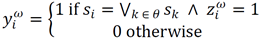
One of the biggest obstacles to human-computer interaction is the prevalence of homonyms in many natural languages (i.e. words that are said or spelled the same way but have different meanings). For example, the word "bass" can refer to a musical instrument, or a freshwater fish. In general, humans are very good at figuring out the meaning of ambiguous words; however, the automatic disambiguation of words remains a difficult task for computers.
Word sense disambiguation (WSD) is one of the central topics of NLP [2]. WSD consists of automatically finding the correct meaning of an ambiguous word in a text, simply by analyzing the context in which it exists. Current WSD methods can be classified into four categories [3]: supervised, unsupervised, semi-supervised, and knowledge-based.
Supervised methods are characterized by the employment of machine-learning techniques, for the purpose of creating classification models based on a training set of hand-labeled corpus that indicates the correct meaning of each ambiguous word in a text. Unsupervised methods do not rely on training; instead, they attempt to provide sense (i.e. meaning) labels by generating clusters of word occurrences. Semi-supervised methods start with a small hand-labeled training set, and progressively improve the classification model, as it is used. Knowledge-based methods make use of knowledge sources such as collocations, thesauri, and dictionaries to assign a sense to an ambiguous word, first by comparing each of its possible definitions with those of other words in the context, and then computing a semantic similarity metric of the definitions.
Knowledge-based methods have recently been proven to outperform supervised approaches in the presence of enough knowledge, or within a knowledge-based domain, while providing at the same time much wider coverage [4].
One of the main challenges of using a dictionary for knowledge-based WSD methods is that the words in the dictionary may be in different forms (e.g., verb, plural, root, etc.), making it difficult to determine the degree of overlap between a word and its respective meanings in the dictionary. To overcome this problem, many of the knowledge-based methods incorporate a stemming step in their algorithms, which consist of reducing inflected (or sometimes derived) words to their word stem, base, or root form.
On the other hand, an associative memory is a computational tool that consists of structures that relate one or more input patterns with an output pattern [5]. One of the foremost properties and fundamental purposes of associative memories is their ability to recall output patterns, despite possible alterations or noise present in input patterns [6]. Associative memories eliminate the exhaustive search operations common in indexed memory, and therefore are very attractive in applications such as data mining and the implementation of sets, where the computations can benefit from the application's specific functioning [7].
Associative memory has been an active topic of research for more than 50 years, and is still investigated both in neuroscience and in artificial neural networks [8]. In particular, Alpha-Beta associative memories have been proven to be a powerful tool for pattern recognition tasks when used in various scientific and technologic applications, such as the classification of patterns in bioinformatics databases [1], prediction of contaminant levels [10], image encryption [11], and translation of Spanish to English [5].
In this paper, we present a method that employs Alpha-Beta associative memory types Max and Min to determine how related each definition of a word is to its context, and then choose the correct definition or sense. Our method was tested using the dataset for the SENSEVAL-2 "All-words" task, with WordNet as the lexical resource. Six different experiments were made, four of them not using a back-off strategy and the remaining two, using it. A back-off strategy is an alternative method that takes a decision when the principal method cannot; the most common strategies used in WSD are: random sense, and most frequent sense. For our purposes we use random sense, because is considered an unsupervised method.
Moreover, to measure the performance of the six different experiments, three statistical metrics were used: precision, recall, and F1-score. All of them were used when our method does not implement a back-off strategy, conversely, when it was used, we only report the F1-score. The latter given that, when a method always take a decision (i.e. the coverage is one hundred percent), the precision, recall, and F1-score are the same.
The rest of the paper is organized as follows: Section II presents the background and related work of simplified Lesk and Alpha-Beta associative memories. Section III presents our proposed method to replace overlapped metric. Section IV describes the experimental resources and results, and in Section V, conclusions derived from the experimental analysis are presented.
II. B and Related Work
A. Simplified Lesk Algorithm
One of the most popular knowledge-based methods for WSD is the Lesk algorithm [12], which is based on the assumption that words occurring in a given section of text will tend to share a common topic. This method consists of obtaining definitions in a dictionary for each word in a given text, and computes the relatedness between all those definitions. The definitions with the greatest relatedness are chosen as the correct senses of the words.
Since the Lesk algorithm may be computationally expensive, a simple Lesk algorithm was proposed [13]. In this method, the meaning of a word is determined by locating the sense that overlaps the most between the definition of the word in a dictionary, and neighboring words (context) of the ambiguous word. In this approach, each word is processed individually and independently of the meaning of other words occurring in the same context.
B. Alpha-Beta Associative Memories
An associative memory is conceived as a system that associates an input pattern (x) with an output pattern (y), through a series of steps known as the learning phase building matrix (M); on the contrary, to retrieve the input's corresponding output pattern, we present the input pattern to the matrix according to the recall phase. The k-th associations are stored in the matrix (M) and its ij-th component is denoted by mij .
The associative memory M is built from a finite set of pre-associated patterns, known as the fundamental set, and is expressed as follows:
 (1)
(1)
p being the cardinality of the fundamental set. Each pattern in the fundamental set is called a fundamental pattern.
There are two categories for an associative memory: if it holds for all fundamental patterns that the input and output patterns to be associated are equals, then the memory M is auto-associative, i.e. xμ≠yμ ∀µ ∈ {1, 2, ..., p}. Otherwise, if there exists one association where the input pattern is different from the output pattern, then the memory M is called hetero- associative i.e. ∃μ ∈ {1, 2, ..., p}, for which xμ≠yμ.
One of the most important characteristics of an associative memory is its ability to deal with a distortion or altered version of the input vectors. It is expected that, if an altered fundamental input vector (
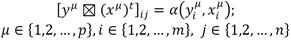
According to [14], the Alpha-Beta model presents two binary operators designed specifically for these memories. First, we defined the sets A = {0, 1} and B = {0, 1, 2}, and operators α and β are defined in Table 1. The sets A and B, the α and β operators (see Table I), along with the usual ∧ (minimum) and ∨ (maximum) operators, form the algebraic system (A, B, α, β, ∧, ∨) which is the mathematical basis for the Alpha-Beta associative memories. This system presents two types of memories: Alpha-Beta associative memory types Max and Min; its name, functionality, and capacity to deal with altered patterns depend on the use of minimum or maximum operators in both learning and recalling phases.

The building of both Max and Min associative memories is denoted by the operator
 (2)
(2)
C. Alpha-Beta Heteroassociative Memories with correct recall
Alpha-Beta heteroassociative memories, unlike the original [14] model and others [15], guarantee the correct recall of the fundamental set [16]. In the following sections, we present the Alpha-Beta heteroassociative memory types Max and Min, with which the complete recall of the fundamental set is guaranteed [16].
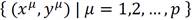
Let A = {0,1}, n, p ∈ Z+, μ ∈ {1, 2, ..., p}, i ∈ {1, 2, ..., p} and j ∈ {1, 2, ..., n}, and let x ∈ An and y ∈ Ap be input and output vectors, respectively. The corresponding fundamental set is denoted by {(xμ , yμ) | μ = 1, 2, ..., p}.
C.1. Alpha-Beta Heteroassociative Memories type Max
Learning phase
The fundamental set must be built according to the following rules: first, all y
vectors must be built according to the one-hot codification, assigning for
yμ the following values:
Step 1: For each
Step 2: Apply the binary
 (3)
(3)Recalling phase
Step 1: Present pattern
 (4)
(4)
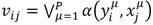
Step 2: It is necessary to build a max sum vector s according to Equation 5:
 (5)
(5)
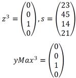
Therefore, the corresponding
 (6)
(6)
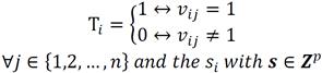
where
C.2. Alpha-Beta Heteroassociative Memories type Min
Learning phase
The fundamental set must be built according to the following rules: first, all y
vectors must be built according to the zero-hot codification,
assigning for yμ the following values:
Step 1: For each
Step 2: Apply the binary
 (7)
(7)
Recalling phase
Step 1: Present pattern
 (8)
(8)
 (9)
(9)
Therefore, the corresponding
 (10)
(10)
where
III. Proposed Algorithm
Considering that inflectional and derivational forms of words affect the process of word sense disambiguation, we propose an algorithm that diminishes the influence of those syntactic phenomena present in the simple Lesk algorithm.
The proposed method replaces the overlap method used in the original simple Lesk algorithm (with the use of Alpha-Beta associative memory types Max and Min), providing one with the ability to deal with an altered version of the words. The following steps show the process of building an associative memory per sense (i.e. one Max and one Min). In the learning phase, the words in the definition of an ambiguous word are used as a fundamental input pattern. Once the memories are built, to assign a sense to an ambiguous word, the context words (which may be an altered version of any fundamental input pattern) are presented to each pair of memories. At the end, a voting strategy applied to the output patterns is used to assign a correct sense.
For example, take the sentence, "The man plays an instrument in a band". To disambiguate the word play, then:
1. The surrounding words and definitions (glosses) are separated in different sets of words, one representing the context and the remaining sets (as many sets as there are meanings for the ambiguous word) corresponding to the senses of the ambiguous word. For this example, we only use the first three senses of the ambiguous word:
C1 = {instrument, band, man}
S1 = {game, sport, hocky, afternoon, cards}
S2 = {act, have, effect, specified}
S3 = {music, instrument, band, night}
2. Due to the binary domain of associative memory operators, the words in the senses, and the context words, are mapped to their corresponding binary representation; for simplicity, we used the ASCII code.
C1 = {
c1 = (0110100101101110011100110111010001110010011 1010101101101011001010110111001110100),
c2 = (01100010011000010110111001100100),
c3 = (011011010110000101101110) }
S1 = {
x1 = (01100111011000010110110101100101),
x2 = (0111001101110000011011110111001001110100),
x3 = (0110100001101111011000110110101101111001),
x4 = (0110000101100110011101000110010101110010011 01110011011110110111101101110),
x5 = (0110001101100001011100100110010001110011) }
S2 = {
x1 = (011000010110001101110100),
x2 = (01101000011000010111011001100101),
x3 = (011001010110011001100110011001010110001101110100),
x4 = (01110011011100000110010101100011011010010110 0110011010010110010101100100) }
S3 = {
x1 = (0110110101110101011100110110100101100011),
x2 = (01101001011011100111001101110100011100100111010101101101011001010110111001110100),
x3 = (01100010011000010110111001100100),
x4 = (0110111001101001011001110110100001110100) }
3. In order to have vectors with the same dimensions, the missing components are filled with zeros or ones depending on the Alpha-Beta associative memory used, zeros for Max types and ones for Min types. In this example, we filled them with zeros.
C1 = {
c1 = (01101001011011100111001101110100011100100111010101101101011001010110111001110100),
c2 = (01100010011000010110111001100100000000000000000000000000000000000000000000000000),
c3 = (01101101011000010110111000000000000000000000000000000000000000000000000000000000) }
S1 = {
x1 = (01100111011000010110110101100101000000000000 0000000000000000000000000000),
x2 = (01110011011100000110111101110010011101000000 0000000000000000000000000000),
x3 = (01101000011011110110001101101011011110010000 0000000000000000000000000000),
x4 = (01100001011001100111010001100101011100100110 1110011011110110111101101110),
x5 = (01100011011000010111001001100100011100110000 0000000000000000000000000000) }
S2 = {
x1 = (0110000101100011011101000000000000000000000 00000000000000000000000000000),
x2 = (0110100001100001011101100110010100000000000 00000000000000000000000000000),
x3 = (0110010101100110011001100110010101100011011 10100000000000000000000000000),
x4 = (0111001101110000011001010110001101101001011 00110011010010110010101100100) }
S3 = {
x1 = (0110110101110101011100110110100101100011000000000000000000000000000000000000 0000),
x2 = (0110100101101110011100110111010001110010011101010110110101100101011011100111 0100),
x3 = (0110001001100001011011100110010000000000000000000000000000000000000000000000 0000),
x4 = (0110111001101001011001110110100001110100000000000000000000000000000000000000 0000) }
4. For each sense, two fundamental sets are built: one according to the associative memory type max (C.1), and one for the associative memory type Min (C.2). Each word in the sense is considered as a fundamental input pattern.
Input vectors:
Sense1 = { x1, x2, x3, x4, x5}
Sense2 = { x1, x2, x3, x4}
Sense3 = { x1, x2, x3, x4}
Output vectors for type Max:
Sense1 = { yMax1 = (10000)t, yMax2 = (01000)t, yMax3 = (00100)t, yMax4 = (00010)t, yMax5 = (00001)t }
Sense2 = { yMax1 = (10000)t, yMax2 = (01000)t, yMax3 = (00100)t, yMax4 = (00010)t }
Sense3 = { yMax1 = (10000)t, yMax2 = (01000)t, yMax3 = (00100)t, yMax4 = (00010)t }
Output vectors for type Min:
Sense1 = { yMin1 = (01111)t, yMin2 = (10111)t, yMin3 = (11011)t, yMin4 = (11101)t, yMin5 = (11110)t }
Sense2 = { yMin1 = (0111)t, yMin2 = (1011)t, yMin3 = (1101)t, yMin4 = (1110)t }
Sense3 = { yMin1 = (01111)t, yMin2 = (10111)t, yMin3 = (11011)t, yMin4 = (11101)t}
Six different fundamental sets are built, two per sense.
Sense 1
FSS1Max = { (x1,yMax1), (x2,yMax2), (x3,yMax3), (x4,yMax4), (x5,yMax5) }
FSS1Min = { (x1,yMin1), (x2,yMin2), (x3,yMin3), (x4,yMin4), (x5,yMin5) }
Sense 2
FSS2Max = { (x1,yMax1), (x2,yMax2), (x3,yMax3), (x4,yMax4) }
FSS2Min = { (x1,yMin1), (x2,yMin2), (x3,yMin3), (x4,yMin4) }
Sense 3
FSS3Max = { (x1,yMax1), (x2,yMax2), (x3,yMax3), (x4,yMax4) }
FSS3Min = { (x1,yMin1), (x2,yMin2), (x3,yMin3), (x4,yMin4) }
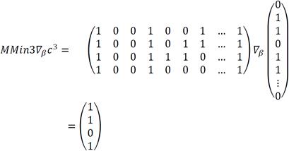
5. For each fundamental set, the corresponding associative memory types Max and Min are built according to step 2 of sections C.1 and C.2 of their respective learning phases. At the end, two associative memories have been built for each sense. We show the building of the matrices corresponding to the third sense (MMax3 and MMin3).
Step 1:

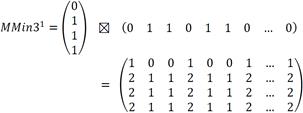
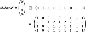


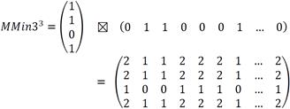
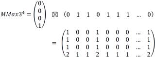


The learning matrices MMax1, MMin1, MMax2, MMin2 are computed in the same fashion.
6. In order to assign a sense to an ambiguous word, its context words are presented to each pair of associative memories. Given that each associative memory corresponds to a sense, the resulting output vectors represent the relation of the context word with said sense. In this example, we present c3 vector to the MMax3 and MMin3 matrices.
Step 1 Max:


7. To adjust the resulting output vectors, derived from the recall phase of the associative memory type Min (in correspondence to the output vectors from associative memory type Max), all their components are negated. This is, a zero value is exchanged for 1, and vice versa.

8. For all output vectors related to each learning matrix, the sum of all components equal to 1 are computed (voting):
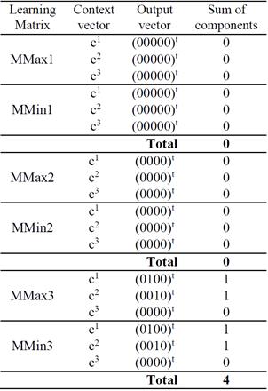
9. The sense corresponding to the learning matrix that has the greatest votes is selected as the correct sense. If more than one sense is selected, then the method is considered unable to determine the sense for the ambiguous word. In this example, the sense selected for the ambiguous word, with a score of four, is the third sense.
IV. Experiments
The performance of the proposed algorithm was assessed using a semantically annotated corpus for SENSEVAL-2 English all-words task [17], and it was compared with results from the simple Lesk algorithm.
SENSEVAL-2 is a dataset that consists of three documents with 2,456 words in 238 sentences. It consists of three tasks: 1) "all-words", "lexical sample", and "translation task". Our comparison is extracted from performances on the "all-words" task. Our proposal, as with any other knowledge-based algorithm, uses a machine-readable dictionary; in this case, we used WordNet.
To measure the performance of the two algorithms, the statistical metrics precision, recall, and F1-score were employed. They are statistical measures that evaluate several aspects of the algorithms [18].
Precision indicates the fraction of retrieved instances that are relevant. This is determined by the number of correct answers, divided by the number of answers given by the algorithm.
Recall is the fraction of relevant instances that are retrieved, and is computed by the number of correct answers, divided by the total number of words for which there is an answer.
F1-score is considered as a weighted average of precision and recall. It is determined by (2PR) / (P + R).
Then, for each sentence in the corpus, and for each word in the sentence, the word to be evaluated (the ambiguous word) is separated from the surrounding words (context). Usually, the senses of each word are expressed in a dictionary (WordNet), as a definition or gloss. In addition to the gloss, there is other information that could be used as an addendum to increase the performance of the disambiguation algorithms. Examples of such information are Synonyms (Syns) and Hyponyms (Hypo). The former, are sets of words that have similar meanings, the latter is a set of more specific synonyms.
Four different experiments were prepared using the information source mentioned before:
1) Gloss (G): only the information of the gloss
2) Gloss + Syns (G+S): the synonyms of the ambiguous word added to its own gloss.
3) Gloss + Hypo (G+H): the hyponyms of the ambiguous word added to its own gloss.
4) Gloss + Syns + Hypo (G+S+H): The gloss of the word added to the hyponyms and synonyms.
V. Results and Discussion
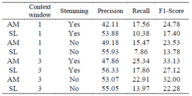
Tables II, III, IV, and V show the results of different experiments, comparing our implementation of the simple Lesk algorithm (SL) against the proposed method (AM). The experiments were developed using two parameters as variables: context window and stemming. It is worth noting that the algorithms presented in these tables did not use a back-off strategy.

The context window is the number of sentences used to disambiguate a word. The possible values for this are: one sentence (which is where the ambiguous word is), and three sentences (the sentence where the ambiguous word is, the one after, and the one before). There are two special cases in context selection: a) when the ambiguous word is in the first sentence, and b) when it is in the last sentence. For both cases, only two sentences are considered: in the first sentence, the window is composed using the sentence with the ambiguous word and its following one. For the last sentence, the context window is the sentence with the ambiguous word and its preceding one. For each configuration, precision, recall, and F1-score were computed.
On the other hand, stemming represents the reduction of a word into a base form. This reduction could be applied (or not) to the context and ambiguous words before the disambiguation process.
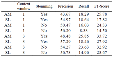
Tables II and III show the experiments using the gloss (Table II), and gloss and synonyms (Table III), as the source of information to form the fundamental set of associative memories. Both tables show that in the precision metric the simple Lesk algorithm performs better than our proposal in each experiment; this means that the simple Lesk algorithm is more assertive when assigning a sense to a word. However our proposal assigns a sense to more words, according to the recall results. In addition, our proposal presents better results as tested using F1-score metric. We can thus conclude from these results that: a) considering the tradeoff between precision and recall, our proposal performs better, and b) our proposal is less dependent on the stemming process, given that the differences between F1-score with and without stemming are smaller than the ones reported from using the simple Lesk algorithm.
Table IV reports the results of when the fundamental set was constructed using the gloss and hyponyms. It shows that each metric had a better performance compared with the ones presented in Table II and III, maintaining observed patterns. This is, the simple Lesk outperforms our proposal in precision, but our proposal performs better in recall and F1-score. In addition, it is worth noting that the AM with a context window of three, without stemming, surpasses the SL in precision.
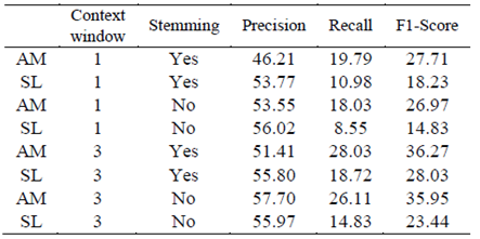
Table V presents the results of when the fundamental set was the compound of the gloss, synonyms, and hyponyms. As opposed to Table III and IV, which present an increased performance when more information was included in the fundamental set, Table V presents a decrease in performance of all simple Lesk experiments in relation to Table IV, whereas just one AM experiment shows this performance decrement. Moreover, as is the same as Table IV, the AM presents a better performance in all F1-scores and presents one case where the AM precision is better than the simple Lesk Algorithm.
Meanwhile, Table VI shows the results of different experiments, comparing the SL algorithm against AM using random sense as a back-off strategy. The F1-score was computed for each information source (G, G+S, G+H, G+S+H), using one and three sentences as context window, and with or without stemming. These experiments exhibit that the AM algorithm does not outperform the SL algorithm for all cases but one, when the context window size is one sentence, without using stemming, and "G+H" as information source, being the F1-score of 45.98.

On the other hand, Table VII presents the results of the AM algorithm compared with two state-of-art algorithms, the random base line (RBL), and the simple Lesk algorithm. The state-of-art algorithms are: 1) a modified implementation of simple Lesk algorithm which instead of selecting the neighboring sentences as context window, it builds its own context by selecting the words that do overlap at least in one word with any gloss of the target word [19]; and 2) a word sense disambiguation algorithm based on Bayes' theorem which compute the a posteriori probabilities of the senses of a polysemous word, then, the sense selected for a given ambiguous word is that with the greater probability [20] (hereinafter Modified SLA and NaiveBayesSM, respectively). These results show that the AM performs better in three out of four algorithms presented, but it is below to Modified SLA which presents an F1-score of 47.8.

VI. Conclusions and Future Work
Tables II to V present, among others metrics, the F1-scores computed for both the associative memory and the original simple Lesk approach. These show that the AM performs better than the simple Lesk algorithm in all cases. In respect to the precision metric, even when the simple Lesk algorithm performs better than our proposal, Tables IV and V show two cases where the associative memory approach outperforms it. These two cases share a context window size of three (the greatest size presented in this work), and the stemming process was not applied. From this, it may be aptly concluded that, in contrast to the simple Lesk algorithm, the associative memory approach is beneficial when more information is available. Furthermore, its performance is not severely reduced when stemming is not applied.
On the other hand, Tables IV and V present interesting outcomes: it seems that, the more data entered in the simple Lesk algorithm for the "bag of words", the more its precision was decreased. If, for both tables, the experiments that correspond to equal size context window -with the same stemming option- are compared, we notice that the simple Lesk algorithm has a reduced precision, if the gloss, synonyms, and hyponyms conform to the bag of words.
Subsequently, Table VI show that when applying the random sense back-off strategy, the SL reports a greater F1-score except for one instance. It is important to note however, that most of the cases where the SL performs better (Table VI) are those where the SL without back-off strategy (Table V), presented a bigger F1-score difference between both algorithms. Therefore, it is possible to infer that when combining a back-off strategy with the SL algorithm, the smaller the F1-score, the fewer decisions are taken by it, then, the back-off randomly choose a sense, and, if the target word has a few senses, it is more likely select the correct one; improving the overall performance. The only instance where the AM comes out better is that where F1-score presents a shorter difference between AM and SL (Table V).
Finally, even when random sense back-off strategy is combined with AM, it does not succeed over Modified SLA. It may be because of the words with which the context are built, are those that appear, at least, one time in any gloss of the word to disambiguate; being more likely selecting the correct sense when the gloss shares one word than those that does not.
In future work, a search for different binary codifications will be made; then, their corresponding implementations will be tested to find the codification that best fit the disambiguation purposes. Another interesting approach to research involves changing the lexical resources (dictionaries), and performing a set of experiments to identify the advantages and disadvantages that are present in each of them. Also, it would be interesting to combine the context building strategy presented by Viveros-Jimenez et al. [19] with our proposal. Finally, in order to increase the response time of the algorithm, a CUDA implementation of our proposal will be made.
In addition, on our future work we plan to explore the role of our WSD method in important tasks where the meaning of ambiguous words plays an important role, such as sentiment analysis [21], [22], [23], sarcasm detection [24], and textual entailment [25].

