


 nueva página del texto (beta)
 Inglés (pdf)
 Artículo en XML
 Referencias del artículo
 Enviar artículo por email
 Citado por SciELO
  Similares en
SciELO
Similares en
SciELO 
 Permalink
I. Introduction
Sensor systems have significant potential for aiding scientific discoveries by instrumenting the real world. For example, the sensor nodes in a wireless sensor network can be used collaboratively to collect data for the purpose of observing, detecting and tracking scientific phenomena. Sensor network deployment is becoming more commonplace in environmental, business and military applications. However, sensor networks are vulnerable to adversaries as they are frequently deployed in open and unattended environments. Anomaly detection is a key challenge in ensuring both the security and usefulness of the collected data. In this paper, we propose a method to filter the compromised nodes, be it self-healing or corrupted, using an autoregressive hidden Markov model (AR-HMM).
The paper is organized as follows. In the next Section II we cover the literature review for this work. In Section III, we give a brief overview of AR-HMMs. In Section IV, we describe the proposed algorithm, and in Section V we give numerical results. The conclusions are given in Section VI.
II. Related Work
Hidden Markov models and the Baum-Welch algorithm were first described in a series of articles by Leonard E. Baum and his peers at the Institute for Defense Analysis in the late 1960s [1]. However detecting compromised nodes using AR-HMM is a new area of investigation and we were unable to find any references that researched the same. Hence we provide the literature review in two parts, first, how compromised nodes are currently filtered and second, on the use of AR-HMM for solving diverse problems of identification, filtering, and prediction.
Wang & Bagrodia [2] have designed an intrusion detection system for identifying compromised nodes in wireless sensor networks using common application features (sensor readings, receive power, send rate, and receive rate). Hinds [3] has used Weighted Majority voting algorithm to create a concept of a node which could not be compromised, and to develop detection algorithms which relied on the trustworthiness of these nodes. Li, Song and Alam [4] have defined a data transmission quality function which keeps close to constant or change smoothly for legitimate nodes and decreases for suspicious nodes. The final decision of whether or not a suspicious node is compromised is determined by a group voting procedure. These designs take the en-network detection approach: misbehaved nodes are detected by their neighboring watchdog nodes. However en-network designs are insufficient to defend collaborative attacks when many compromised nodes collude together in the network. Zhang, Yu and Ning [5] present an alert reasoning algorithm for intelligent sensors using cryptographic keys. Zhanga et al. [6] exploit a centralized proven collision-resilient hashing scheme to sign the incoming, outgoing and locally generated/dropped message sets. These algorithms work on pinpointing exactly where the false information is introduced and who is responsible for it, but they are centralized and do so at a high computational cost. We propose a simple, decentralized model based approach to identify compromised nodes at a low computational cost using HMMs.
HMMs have been successfully used to filter unreliable agents, see Chang & Jiliu [7], Anjum et al. [8]. However the approach is unable to model correlation between observations. Autoregressive HMMs alleviate this limitation. Introduced in the 1980's, Juang and Rabiner published a series of papers [9], [10] regarding the application of Gaussian mixture autoregressive HMM to speech recognition. Switching autoregressive processes are well understood and have been applied in many areas. They have been particularly popular in economics, see Alexander [11] and Hamilton [12]. A brief summary of this subject and an extensive list of references can be found in [13]. The model is also successfully used by Park, Kwon and Lee [14], they have used AR-HMM by modeling the probabilistic dependency between sequential target appearances, presenting a highly accurate algorithm for robust visual tracking.
III. Proposed Model using Autoregressive Hidden Markov Models
A hidden Markov model is a Markov Chain with N states, which are hidden from the user. When the Markov chain is in a state, it produces an observation with a given state-dependent probability distribution. There are M different observation paths. It is this sequence of observations that the user sees, and from which it is possible to estimate the parameters of the HMM. An HMM is defined by the A matrix which is the one-step transition matrix of the Markov chain, the B matrix (referred to as the event matrix) which contains the probability distribution of the observations likely to occur when the Markov chain is in a given state, and π, the vector of probabilities of the initial state of the Markov chain. The (A, B, π) are together represented by λ. In this paper, we will make use of the following notation:
A: One-step transition Matrix (N x N)
aij : One-step probability from state i to state j
B: Event Matrix (N x M)
bi (k): Probability that the kth value will be observed when system shifts to state i
π: Initial Probability vector (N x 1)
N: Number of hidden states
M: Number of observations
O: An observation sequence
T: Length of the observation sequence
Q: A sequence of hidden states traversed by the system
λ = (A, B, π)
A useful extension of HMM is autoregressive HMM (AR-HMM), which enhances the HMM architecture by introducing a direct stochastic dependence between observations. In AR(p)-HMM, the observation sequence is not only dependent on the HMM model parameters but also on a subset of p previous observations. Thus the model switches between sets of autoregressive parameters with probabilities determined by a state of transition probability similar to that of a standard HMM:
where ar(st) is the rth autoregressor when in state s ∈ {1 ... N} at time t and each ƞt is an i.i.d. normally distributed innovation with mean 0 and variance σ2. Observations in the general AR-HMM can be continuous, but for our purposes we restrict the discussion to the discrete case. For example, a discrete HMM with AR(1) can be depicted by the Directed Acyclic Graph (DAG) as shown in Fig. 1. Three different, but related, problems have been defined for HMMs, briefly described below.
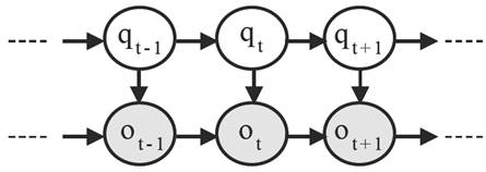
Fig. 1 DAG of the AR(1)-HMM where qi and oi represent the state and the observation generated at time slot i respectively.
Problem 1: Forward Probability Computation: Given an observation sequence, compute the probability that it came from a given λ.
Let the system be in state i at time t. The probability of
the system shifting to state j at t+1 is given
by the one-step transition probability aij
. The probability that of the M possible observed
states, the kth one is observed given that the system shifted
from state i to j is
aijbj(k). Since
the state i can be any one of the states from 1 to
N, the probability of observing the kth
value, given that the system shifts to state j at time
t+1 is the sum of all probable paths to state
j, i.e.,
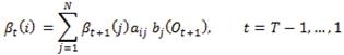
Now, the only remaining unknown is the joint probability of having observed the sequence from O1 through Ot and being in state i at time t, given λ. Representing this quantity by αt(i) and representing the kth observed value at time t+1 by Ot+1 , we have

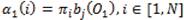
To start off this induction, the initialization step for calculating αt(i) can be obtained as follows. The probability of the system being in state i at time 1 is given by πi and the probability of observing O1 is then given by bj (O1 ). Thus,
αT(i) obtained from the induction step represents the probability of observing the sequence from O1 through OT , and ending up in state i. Thus, the total probability of observing the sequence O1 through OT , given λ is

Problem 2: Backward Probability Computation: Given an observation sequence, compute the probable states the system passed through.
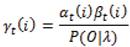
The quantity βt(i) is defined as the probability that the sequence of observations from Ot+1 through OT are observed starting at state i at time t for a given λ. It is calculated in the same way as αt (i), but in the backward direction. We have,

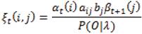
For t = T we have βT (i)=1, i = 1, 2, ..., N. To calculate the probability that the system was in state i at time t given O and λ, we observe that αt (i) accounts for the observation sequence from O1 through Ot and βt (i) accounts for Ot+1 through OT , and both account for the state i at time t. So the required probability is given by αt(i)βt(i). Introducing the normalizing factor from problem 1, P(O|λ), we have
At each time t, the state with the highest γ is the most probable state at time t. A better way to obtain the most probable path of states Q that give rise to an observation sequence O, is to use dynamic programming, as described in [13].
Problem 3: Matrix Estimation: Given an observation sequence O, compute the most probable λ.
The term aij can be calculated as the ration of the number of transitions made from state i to state j over the total number of transitions made out of state i. We have from problem 2 that γt(i) is the probability of being in state i at time t. Extending this, the probability of being in state i at time t and in state j at time t+1 can be calculated as follows:
IV. The Algorithm
We consider a set of sensors that consists of a mix of healthy, self-healing and corrupted sensors. We assume that time is slotted, let T be the total number of slots. During each slot, each sensor submits a reading about the environment. For simplicity, let all the nodes submit a reading at each time slot. (This constraint can be easily removed, by appropriately modifying the way the αi(t) and βi(t) are calculated.)
For each node, we have a sequence of T readings (observations) to train an AR-HMM. Thus, we end up with as many AR-HMMs as the number of nodes. Using statistical clustering techniques, we cluster the B matrices of these AR-HMMs into two groups, one for healthy and the other for compromised nodes (self-healing and corrupted). This permits us to identify and filter out the compromised sensors.
To test the accuracy of the algorithm, we consider three types of sensors, healthy, self-healing and corrupted. To achieve this, we define three λ's, all having the same A and π, but different B. The B matrix of the healthy nodes (Bh ) should be such that the readings generated echo the environmental phenomenon it is sensing. The B matrix of self-healing nodes (Bs ) introduces spurs of invalid data before moving back to the valid state and the B matrix of the corrupted nodes (Bc ) is set up to predominantly generate invalid data. The exact matrices are defined in the next section.
Next, this sequence of T readings is used to estimate the A, B, and π matrices of the sensor. Using the B matrices, we cluster the sensors into two groups, i.e., healthy and compromised nodes. For this, we take the mean squared error (MSE) of each estimated B matrix with the perfectly healthy matrix Bp (see Section IV), where

and bi(k) and bpi(k) are the (i,k)th element of the B and Bp matrices respectively.
The resulting MSE values are then classified into two clusters using the k-means clustering algorithm. As Bp represents the truly healthy matrix, the cluster with a center closer to 0 represents the group of healthy nodes.
V. Experimental Setup and Results
A. Synthetic Datasets - Richardson's Model
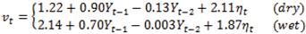
For our simulation study, we use the classic Richardson's model for the temperature [14] to define the transition matrix A and the autoregressors vi . Richardson's model uses two states St = {Dry, Wet}, hence N = 2, and second order autoregression, AR(2), to define the temperature readings. The model is given as follows:

The results reported in this section were based on 60% healthy nodes, 20% self-healing, and 20% corrupted nodes. In all experiments, we set the Markov chain to start with an equal probability of being in any of the two hidden states, i.e., π = [0.5, 0.5]. We define three B matrices (Bh, Bs and Bc), such that they model the behavior of the three nodes under consideration, healthy, self-healing and corrupted respectively. B is a 2 x 2 matrix where the first column corresponds to the probability of generating a value using autoregressive equations, and second column corresponds to the probability of entering the corrupted state and generating an invalid value. (The selection of N = M = 2 is not significant, and any other values can be readily used).

The perfectly healthy matrix, Bp used for MSE calculations is defined as

For the above A matrix, we define three AR(2)-HMMs, namely, λh = (A, Bh, π), λs = (A, Bs, π) and λc = (A, Bc, π).. Subsequently, we generate random samples of temperature readings for all the nodes, and then apply the algorithm described in the previous section to identify the group of healthy nodes. Then, we compare the number of identified healthy nodes to the original set of healthy sensors and report the result as a percentage of correctly identified healthy nodes. We used MS_Regress MATLAB package for Markov Regime Switching Models by Perlin [15] to implement the above algorithm and obtain numerical results.
The results are given in Fig. 2 which gives the percentage of correctly identified healthy (left) and corrupted (right) nodes along with the 95th confidence interval. For the figure, we assume 10, 50 and 100 sensors, and vary the number of observations per sensor from 10 to 50. The confidence intervals are obtained by replicating each result 100 times, and each time using a different seed for the pseudo-random number generator.
Interesting observations (Fig. 2): As the number of readings increases per node, the prediction accuracy the nodes (both healthy and corrupted) increases as well. For healthy nodes, the average prediction accuracy for 10 readings is around 88% and for 50 readings per node, it jumps to around 97%. Overall, the prediction accuracy of healthy nodes is much higher than that of corrupted nodes. This can be explained by the fact that the cluster distribution of self-healing nodes and corrupted nodes is quite similar whereas both differ significantly from the cluster distribution of healthy nodes.
Based on the results, we also observe that it is not necessary to have a large sample of nodes and readings per node. We see that with as little as 10 nodes and 10 readings per node, we obtain results which are similar to those obtained with larger number of nodes and readings per node. This leads us to conclude that our approach can be used in a decentralized manner, i.e., we do not need data from all (or a large number) of the sensors in order to prune out the compromised ones.
Finally, we turn towards sensitivity analysis of our approach, i.e., how does the percentage of self-healing nodes impact the filtering accuracy. For this we varied the percent of self-healing nodes from 0 to 50%. Keeping the number of nodes to 50 and the number of readings per node to also 50, we calculate the prediction accuracy of the healthy and corrupted nodes. The results are presented in Table I.
We make the following observations. As the number of self-healing nodes increases, the prediction accuracy of both healthy nodes and corrupted nodes decreases. However, where the change in healthy node prediction is minor (98% to 95%), corrupted node prediction suffers increasingly as the number of self-healing nodes increases (95% to 68%). This confirms our initial observation that the cluster distribution of self-healing nodes is similar in nature to corrupted nodes. Hence it becomes difficult for the algorithm to pick corrupted nodes exclusively from the set of corrupted and self-healing nodes. The success of our approach, however, lies with the identification of healthy nodes, with accuracy greater than 90%.
B. Real Sensor Datasets
In order to test our models on real world sensor datasets, we use datasets from two sources: Intel Berkley Research Laboratory [16] and Labeled Wireless Sensor Network Data Repository (LWSNDR) projects [17]. Both projects represent the state of the art in sensor systems and collect measurements in very different environments. Hence, these datasets allow us to evaluate the accuracy of AR-HMM classification on representative and diverse sensor system data.
First dataset is collected from 54 sensors deployed in the Intel Berkeley Research lab. The Mica2Dot sensors with weather boards collected time stamped topology information, along with humidity, temperature, light and voltage values once every 31 seconds. This dataset includes a log of about 2.3 million readings collected from the 54 motes (mote is a sensor that is capable of doing some processing in addition to collecting and transmitting data), where data from some motes may be missing or truncated.
Second dataset is collected from a simple single-hop and a multi-hop wireless sensor network deployment using TelosB motes. The data consists of humidity and temperature measurements collected during 6 hour period at intervals of 5 seconds. For this evaluation, we are using the single hop labeled readings which consist of approximately 15,000 entries.
The first dataset is unlabeled. We have tested our anomaly detection algorithms with by visually inspecting the sensor data time series. The second dataset, is a labelled wireless sensor network dataset where label '0' denotes normal data and label '1' denotes an introduced event (anomaly). More details can be obtained from [18].
We assume that the sensor readings collected over a reasonable duration capture the normal patterns in the sensor data series. As a general rule, we have used 20% of the data points to work out the auto regression equations for the system. The auto regressive coefficients are calculated using the least squares method. Also, the same data points are used to calculate λ = (A, B, π) as defined under Problem 3 in Section 2.
For comparison, we are using two popular classification algorithms ZeroR and Naïve Bayes along with our proposed AR-HMM model. Briefly, ZeroR is a useful predictor for determining a baseline performance, predicting mean for a numeric class and mode for a nominal class, and Naïve Bayes is a conditional probabilistic classifier based on Bayer's theorem. The filtering accuracy to identify healthy nodes is given in Table II.
Table II displays that as ZeroR provides a baseline accuracy, AR-HMM clearly surpasses Naïve Bayesian classification for correctly identifying the healthy sensors. We further describe our method's accuracy using (1) number of false positives (detecting non-exist compromised nodes) and (2) number of false negatives (not being able to detect a compromised node) as our metrics. Specifically, the results in Table III below are presented as follows - the x/y number indicates that x out of y compromised nodes were detected correctly (corresponding to y-x false negatives) plus we also indicate the number of corresponding false positives.
VI.Conclusion
In this paper, we propose a method based on autoregressive hidden Markov models (AR-HMMs) for filtering out compromised nodes in a sensor network. We confirm through experimentation, based on revised Richardson's temperature model, that our filtering method is quite accurate and identifies the healthy sensors with an accuracy greater than 90%. We further used real sensor data from Intel Labs and WSN repository from UNC to calculate the prediction accuracy of AR-HMM approach as opposed to Naïve Bayes and ended up with encouraging results, with prediction accuracy as high as 97%

