


 nueva página del texto (beta)
 Inglés (pdf)
 Artículo en XML
 Referencias del artículo
 Enviar artículo por email
 Citado por SciELO
  Similares en
SciELO
Similares en
SciELO 
 Permalink
I. Introduction
PCA is a way of identifying patterns in data, and expressing the data in such a way as to highlight their similarities and differences. Since patterns in data can be hard to find in data of high dimension, where the luxury of graphical representation is not available, PCA is a powerful tool for analyzing data. The other main advantage of PCA is that once we have found these patterns in the data, then we compress the data, i.e., by reducing the number of dimensions, without much loss of information.
PCA and Singular Value Decomposition (SVD) are interchangeably used for data reduction/compressions whereas statistical techniques such as regression analysis are used for approximation and analysis of data. Such applications include data mining, health informatics, oceanography, meteorology, natural language processing, machine learning, image analysis, geometry visualization.
A. Qualitative Spatial Reasoning
Reasoning about spatial data is a key task in many applications, including geographic information systems, meteorological and fluid flow analysis, computer-aided design, and protein structure databases. Such applications often require the identification and manipulation of qualitative spatial representations, for example, to detect whether one "object" will soon occlude another in a digital image, or to determine efficiently relationships between a proposed road and wetland regions in a geographic dataset. QSR provides representational primitives (a spatial "vocabulary") and inference mechanisms.
Much QSR work has studied purely topological descriptions of spatial regions and their relationships. One representative approach, the Region-Connection Calculus (RCC), provides predicates for expressing and reasoning about the relationships among topological regions (arbitrarily shaped chunks of space). RCC was originally designed for 2D [1, 2]; later it was extended to 3D [3]. Herein we introduce PCA to reduce 9-Intersection model to 4-intersection model in both 2D and 3D. The performance of QSR can be improved by reducing the number of intersections, but PCA connection to QSR is non-existent in the literature. Herein we show how (1) PCA can be applied to intersection dimension reduction for QSR spatial data, and (2) the 9-Intersection can be reduced to 4-Intersection for all spatial as well as non-spatial objects.
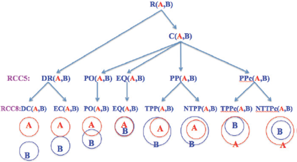
For example, of item-attribute-concept in RCC, spatial objects are items, their intersections are attributes, and relations are concepts. There are five RCC5 and eight RCC8 concepts in RCC, see Figure 1, and [2, 3].
B. Health Informatics
The Big Data revolution has begun for many industries. The healthcare industry has been playing catch up and has finally reached a consensus on the value of Big Data as a transformative tool. Statistical linear and logistic regression that have been the popular mining techniques, but their ability to deal with inter dependent factors is limited. The understanding of principal components, however, has been lacking in the past by non-academic clinicians. It is no surprise that keeping people healthy is costing more money. From the price of medications and the cost of hospital stays to doctors' fees and medical tests, health-care costs around the world are skyrocketing. Much of this is attributed to wasteful spending on such things as ineffective drugs, futile procedures and redundant paperwork, as well as missed disease-prevention opportunities. This calls for mechanism for efficient data reduction and diagnostic tools as pointed out by some of the examples in the literature cited in the next paragraph.
Analysis of this Big Data offers unlimited opportunities for healthcare researchers and it is estimated that developing and using prediction models in the health-care industry could save billions by using big-data health analytics to mine the treasure trove of information in electronic health records, insurance claims, prescription orders, clinical studies, government reports, and laboratory results. According to the Harvard School of Public Health publication entitled The Promise of Big Data, petabytes of raw information could provide clues for everything from preventing tuberculosis to shrinking health care costs-if we can figure out how to apply this data [4]. Improving the care of chronic diseases, uncovering the clinical effectiveness of treatments, and reducing readmissions are expected to be top priority use cases for Big Data in healthcare [5].
In this paper, we will give general guidelines to address various issues. We explore an adaptive hybrid approach (1) how PCA can be used to reduce data in the original space in addition to transformed space, (2) how PCA can be used to improve standard line regression and logistic regression algorithms, (3) how to use logistic regression in conjunction PCA to yield models which have both a better fit and reduced number of variables than those produced by using logistic regression alone.
The paper is organized as follows. Section II describes the background on linear regression, logistic regression, and principle of component analysis. Section III describes PCA in detail, along with our suggested representational improvements. Section IV presents the hybrid algorithms for regression using PCA. Section V discusses PCA's improved role in dimensionality reduction followed by additional experimental support in Section VI. Section VII concludes the paper.
II. Background
A. Mathematical Notation
In this section, we describe the mathematical notation for terms whose definitions will follow in the paper. A vector is a sequence of elements. All vectors are column vectors and are in lower case bold letters such as x. The n-tuple [x 1,..., xn] denotes a row vector with n elements in lowercase. A superscript T is used to denote the transpose of a vector x, so that xT is a row vector whereas x = [x1,..., x n ]T is a column vector. This notation is overloaded at some places where the ordered pair [xl, x2 ] may be used as a row vector, a point in the plane or a closed interval on the real line. The matrices are denoted with uppercase letters, e.g. A, B. For vectors x, y, the covariance is denoted by cov(x, y), whereas cov(x) is used for cov(x, x) as a shortcut [6].
If we have m vector values
x
l;,...,xm
of an n-dimensional vector x = [x
l;,..., xn
]T, these m row vectors are collectively
represented by an m x n data matrix A. The
kth
row of A is the row vector
There are several ways to represent data so that implicit information becomes explicit. For linear representation of vector data, a vector space is equipped with a basis of linearly independent vectors. Usually in data mining, the data is represented as a matrix of row vectors or data instances. Two of the methods for efficient representation of data are regression and PCA.
B. Qualitative Spatial Reasoning
Much of the foundational research on QSR is related to RCC that describes two regions by their possible relations to each other. RCC5/RCC8 can be formalized by using first order logic [2] or by using the 9-intersection model [1]. Conceptually, for any two regions, there are three possibilities: (1) one object is outside the other; this results in the RCC5 relation DR (interiors disjoint) and RCC8 relation DC (disconnected) or EC (externally connected). (2) One object overlaps the other across boundaries; this corresponds to the RCC5/RCC8 relation PO (proper overlap). (3) One object is inside the other; this results in topological relation EQ (equal) or RCC5 relation PP (proper part). To make the relations jointly exhaustive and pairwise distinct (JEPD), there is a converse relation denoted by PPc (proper part converse), PPc(A,B) = PP(B,A). For a close examination, RCC8 decomposes RCC5 relation PP (proper part) into two relations: TPP (tangential proper part) and NTPP (non-tangential Proper part). Similarly for RCC5 relation PPc, RCC8 defines TPPc and NTPPc. The RCC5 and RCC8 relations are pictorially described in Figure 1.
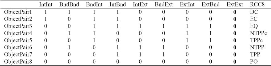
Each of the RCC8 relations can be uniquely described by using the 9-Intersection framework. It is a comprehensive way to look at any relation between two regions. The 9-Intersection matrix for two regions A and B is given in Table 1, where Int represents the region's interior, Bnd denotes the boundary, and Ext represents the exterior. The predicate IntInt(A,B) is a binary relation that represents the intersection between the interiors of region A and region B; the value of this function is either true (non-empty) or false (empty). Similarly, there are other predicates for the intersection of A's interior, exterior, or boundary with those of B. In QSR, we are only concerned with the presence/absence of an intersection. The actual value of the intersection is not necessary.
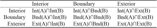
For two non-empty bounded regions A and B, the intersection of their exteriors is always non-empty. This is represented in the last column of Table 2. Since it adds no new information, it has been proposed in the literature [2] to replace the 9-Intersection with the 8-Intersection model to define the spatial relations. The values of the 8-Intersection framework for the RCC8 framework are given in the first eight columns in Table 2.
In this paper, we show that PCA provides a better alternative to conventional methods of dimensionality reduction in QSR. The analysis is equally applicable to both non-spatial discrete web objects as well as conventional spatial objects such as cuboids and spheres.
In such applications, some threshold may be required to interpret the resulting dimensions. one can simply ignore variation below a particular threshold to reduce the data and still preserve the main concepts of original intent.
C. Health Informatics
There is a significant opportunity to improve the efficiencies in the healthcare industry by using an evidence-based learning model, which can in turn be powered by Big Data analytics [7]. A few examples are provided below. The company Asthmapolis has created a global positioning system (GPS) enabled tracker that monitors inhaler usage by patients, eventually leading to more effective treatment of asthma [8]. Center for Disease Control and Prevention (CDC) is using Big Data analytics to combat influenza. Every week, the CDC receives over 700,000 flu reports including the details on the sickness, what treatment was given, and whether not the treatment was successful.
The CDC has made this information available to the general public called FluView, an application that organizes and sifts through this extremely large amount of data to create a clearer picture for doctors of how the disease is spreading across the nation in near real-time [9]. GNS Healthcare, a Big Data analytics company, has come together with the health insurance company Aetna to help combat people at risk or already with metabolic syndromes. The company has developed a technology known as Reverse Engineering and Forward Simulation that will be put to work on the data of Aetna insurance subscribers. Essentially, the technology will search for the presence of five warning signs: large waist size, high blood pressure, high triglycerides, low High density Lipoprotein, and high blood sugar. A combination of any three of these lead to the conclusion that the patient is suffering from the condition [10].
Researchers at Allazo Health are creating systems designed to improve on medication adherence programs by using predictive analytics. For example, predict what interventions are mostly likely to work for that patient based on what interventions already worked for other patients with similar demographics, behavioral profiles, and medical history [11]. Another area of interest is the surveillance of adverse drug reactions (ADRs) which has been a leading cause of death in the United States [12]. It is estimated that approximately 2 million patients in USA are affected by ADRs and the researchers in [13], [14] and [15] propose an analytical framework for extracting patient-reported adverse drug events from online patient forums such as DailyStrength and PatientsLikeMe.
Simplistically speaking, in all the above examples the researchers are trying to model and predict a dependent phenomenon based on a number of predictors that have been observed. The dependent parameter can be discrete, nominal, or even binary / logical. There are two problems at hand: dimension reduction and prediction. First problem is data optimization. The optimization problem is data cleaning, and how we can reduce the set of predictors while still maintaining a high prediction accuracy for the dependent variable. The second problem is the prediction of the dependent variable from the reduced dataset. This problem is analyzing whether some event occurred or not given the success or failure, acceptance or rejection, presence or absence of observed simulators. This is where PCA comes into the picture.
III. Principle Component Analysis
The PCA is a well-known data reduction tool in academia for over 100 years. PCA creates a linear orthogonal transformation of correlated data in one frame (coordinates system) to uncorrelated data in another frame. The huge dimensional data can be transformed and approximated with a few dimensions. PCA finds the directions of maximum variance in high-dimensional data and projects it onto a smaller dimensional subspace while retaining most of the original information. If the data is noisy, PCA reduces noise implicitly while projecting data along the principal components. In this paper, we explore an adaptive hybrid approach to show that PCA can be used not only for data reduction but also for regression algorithm improvement. We will describe the hybrid model for both linear and logistic regression algorithms.
Before delving further, we would like to discuss the terms PCA and SVD further as they are used interchangeably in the literature. There is a clear distinction between them.
Definition 1. For a real square matrix A, if there is a real number λ and a non-zero vector x such that A x = λx, then λ is called an eigenvalue and x is called an eigenvector.
Definition 2. For a real matrix A (square or rectangular), if there a non-negative real number σ and a non-zero vectors x and y such that AT X = σ y, and A y = σx, then σ is called a singular value and x and y represent a pair of singular vectors [16].
Note 1. λ can be negative or positive, but σ is always non-negative.
Note 2. σ2 is an eigenvalue of covariance matrices AAT and AT.A This can be quickly seen
Therefore
Similarly, we can see that
An eigenvector is a direction vector supporting the spread of data along the direction of the vector. An eigenvalue measures the spread of data in the direction of the eigenvector. Technically, a principal component can be defined as a linear combination of optimally weighted observed variables. The words "linear combination" refer to the fact that weights/coefficients in a component are created by the contribution of the observed variables being analyzed. "Optimally weighted" refers to the fact that the observed variables are weighted in such a way that the resulting components account for a maximal amount of variance in the dataset.
This will also be a good place to introduce Least Square Approximation (LSA). LSA and PCA are both linear transformations. However, they accomplish the same task differently. In a vector space, for any vector v and a unit vector u, we have v= v·u u + (v - v·u u). Finding the vector u that minimizes |( v - v·u u)| is the same as finding a vector u that maximizes |v· u|. LSA calculates the direction u that minimizes the variance of data from the direction u whereas PCA computes the direction u (principal component) that maximizes the variance of the data along the direction u. This concept is applied to all data instance vectors collectively resulting in covariance matrix AAT of data matrix and u is the eigenvector of AAT with largest eigenvalue.
If A is a real square symmetric matrix, then eigenvalues are real and eigenvectors are orthogonal [17]. PCA computes eigenvalues and eigenvectors of a data matrix to project data on a lower dimensional subspace. PCA decomposition for a square symmetric matrix A is A = UDUT where U is the matrix of eigenvectors and D is diagonal matrix of eigenvalues of A. Since AU = UD, U is orthogonal, therefore A=UDUT. Also PCA orders the eigenvalues in the descending order of magnitude. The columns of U and diagonal entries of D are arranged correspondingly. Since eigenvalues can be negative, the diagonal entries of D are ordered based on absolute values of eigenvalues.
The SVD decomposition is applicable to a matrix of any size (not necessarily square and symmetric). A = USVT, where U is the matrix of eigenvectors of covariance matrix AAT, V is the matrix of eigenvectors of covariance matrix ATA and S is a diagonal matrix with eigenvalues as the main diagonal entries. Hence, PCA can use SVD to calculate eigenvalues and eigenvectors. Also SVD calculates U and V efficiently by recognizing that if v is an eigenvector of ATA for non-zero eigenvalue λ, then A v is automatically an eigenvector of AAT for the same eigenvalue λ where λ≥0. If A v is an eigenvector, say, u, then A v is a multiple of eigenvector u (since u and v are unit vectors) and it turns out that Av = √λ u , or u = σAv, where σ = 1/ √λ. By convention, SVD ranks the eigenvectors on descending order of eigenvalues. If U and V are matrices of eigenvectors of AAT and ATA and S is the matrix of square roots of eigenvalues on the main diagonal, then A can be expressed as A = USVT [17]. The eigenvalues of a square symmetric matrix A are square roots of eigenvalues of AAT We will show that it is sufficient to have S as diagonal matrix of only non-zero eigenvalues and U, V to have columns of only the corresponding eigenvectors.
In data mining, the m observations/data points are represented as an m x n matrix A where each observation is a vector with n components. PCA/SVD help in transforming physical world data / objects more clearly in terms of independent, uncorrelated, orthogonal parameters.
The first component extracted in principal component analysis accounts for a maximal amount of variance in the observed variables. The second component extracted will have two important characteristics. First, this component will account for a maximal amount of variance in the dataset that was not accounted for by the first component. The second characteristic of the second component is that it will be uncorrelated with the first component. The remaining components that are extracted in the analysis display the same two characteristics. Visualizing graphically, for the first component direction (eigenvector) e1, the data spread is maximum m1; for the next component direction e2, the data spread is next maximum m2 (m2 < ml the previous maximum) and the direction e2 is orthogonal to previous direction e1.
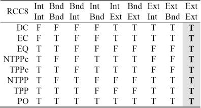
Note 3. For the eigenvectors u of A, any non-zero multiple of u is also an eigenvector of A. In U, the eigenvectors are normalized to unity. If u is a unit eigenvector, then -u is also a unit eigenvector. Thus the sign can be arbitrarily chosen. Some authors make the first nonzero element of the vector to be positive to make them unique. We do not follow this convention. Since the eigenvectors are ordered, we make the kth element of vector u k positive. If kth element is zero, only then first non-zero element is made positive. This is a better representation of eigenvectors as it represents the data in a right-handed system as opposed to asymmetrical ordering, see Figure 2. Using Matlab svd(A) on a simple set of only two data points, the algorithm generates two orthogonal vectors v 1, v2 as given in Figure 2(a, b). our algorithm finds green vectors in Figure 2(c), which is more natural and of a right-handed orientation.
Fig. 2 Gray set of axes are standard xy-system. Blue dots represent a set of data points. Red dots are projections of data points on the principal components. (a) The axes v1, v2 in red are the eigenvectors that are computed by Matlab using the set of data points. (b) The axes v1, v2 in blue are the directions so that each eigenvector is unique making the first non-zero component positive, used in the literature. (c) The axes v1, v2 in green are generated when the sign in an eigenvector is chosen by our scheme.
A. Properties of PCA/SVD
In essence, PCA/SVD takes a high dimensional set of data points and reduces it to a lower dimensional space that exposes the knowledge that is hidden in the original space. Moreover, the transformation makes similar items more similar, and dissimilar items more dissimilar.
It is not the goal of SVD to get back the original matrix. However, the reduced dimensions do give insight about the original matrix, as we will see in the case of QSR and health informatics.
There are three important properties of SVD:
It can transform correlated variables into a set of uncorrelated ones. SVD computes a transformation T such covariance of TA is diagonal matrix D, e.g. TA(TA)T is D. It can extract some relationships hidden in the original data. It can also reduce noise in the data [18].
Since the eigenvectors are ordered on most variation to least variation in descending order of eigenvalues, deleting the trailing eigenvectors of smaller variation ensures minimal error. It finds the best approximation of the original data points by projecting data on a fewer dimensional subspace; see Figure 3 of linear data.
The data can be reduced to any desired size. The accuracy of smaller size data depends on the reduction in the number of dimensions [19]. By deleting eigenvectors corresponding to least variation, we effectively eliminate noise in the representation of data vectors [20].
B. Dimension Reduction using PCA
There is a multitude of situations in which data is represented as a matrix. In fact, most of the real world data is expressed in terms of vectors and matrices where each vector has a large number of attributes. Matrices are used to represent data elegantly, and efficiently. In a matrix, each column represents a conceptual attribute of all the items, and each row represents all attributes related to individual data item. For example, in health informatics, rows may represent patients and columns may represent disease diagnostic symptoms or the rows may represent medicines and columns may represent side effects or adverse reactions. Similarly, in spatial-temporal reasoning, rows represent pairs of objects and columns represent temporal intersection properties of objects.
The goal of PCA is to reduce the big data matrix A to a smaller matrix retaining approximately the same information as the original data matrix and make the knowledge explicit that was implicit in the original matrix.
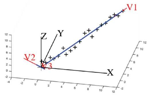
Example: In this example, we have 20 three-dimensional points in 20 x 3 matrix A. Each row of A has three values for x-, y-, z- coordinates. Visually we can see that the data points have a linear trend, in 3D, but data points have noise components in the y, and z coordinates. PCA determines the direction and eliminates noise by eliminating the eigenvectors corresponding to smaller eigenvalues (see Figure 3). Black "+" symbols represent the original data points with noise. As can be seen visually, they are almost linear. They can be approximated along eigenvector v 1 in one dimension of the v1v2v3 -system. Red lines depict the data trend in the three dimensional space along v1, v2 and v3 direction. Blue lines depict the data spread in the three dimensional space along v1, v2 and v3 direction. Since the data spread or blue line on v2 and v3 is almost non-existent (closer to the origin), it is an indicator of noise in the linear data. We can see that the data can be represented satisfactorily using only one direction.
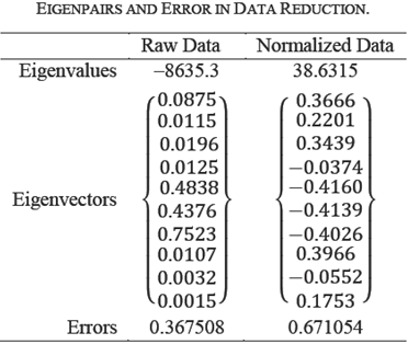
Table 3 enumerates the numeric values of
the PCA decomposition. First row lists the eigenvalues, which represent the
spread of points along the principal components. Second row shows the
eigenvectors corresponding to the eigenvalues. The next three rows represent the
error on using first, first two, first three eigenpairs. Let
newA be the USVT
based on eigenpairs used. Then Error Original is the
|A-newA |/|A| percentage error in the original space. Error
Projection is the |AV-newAV|/|AV| percentage error in the
projection space. Error Eigenvalues is the
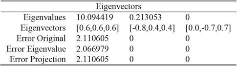
Table 3 reveals that v1, is the data dimension and v2, v3 correspond to the noise in this case. If we use two (or three) eigenpairs there is no error. Hence, the data can be represented in one dimension only instead of three dimensions with slight error of 2%. This error is attributed to the difference between the non-zero eigenvalues. The third and fifth rows in Table 3 indicate that the error metrics are equivalent in the original and projection space.
IV. Principal Component And Regression Analysis
There are several ways to model the prediction variables, e.g., linear regression analysis, logistic regression analysis, and PCA. Each has its own advantages. Though regression analysis has been well known as a statistic technique, the understanding of principles, however, has been lacking in the past by non-academic clinicians [21]. In this paper we explore an adaptive hybrid approach where PCA can be used in conjunction with regression to yield models which have both a better fit and reduced number of variables than those used by standalone regression. We will apply our findings to a medical dataset obtained from UCI Machine Learning Repository about liver patient [22]. We use the records for detecting the existence or non-existence of liver disease based on several factors such as age, gender, total bilirubin, etc.
A. PCA and Linear Regression
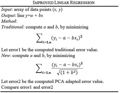
In linear regression, the distance between observed point (xi,yi) from the computed point (xi,a+bxi) on line y=a+bx, is minimized along the y direction. In PCA, the distance of the observed point (xi,yi) is minimized to a line which is orthogonal to the line y=a+bx, is minimized. The details of linear algebra concepts in this section are found in [17]. We assume that data is standardized to mean zero; and normalized appropriately by the number of objects.
For one independent and one dependent variable, the regression line is y=a+bx where the error between the observed value yi and estimated value a+bxi is minimum. For n points data, we compute a and b by using the method of least squares that minimizes:
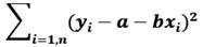
This is a standard technique that gives regression coefficients a and b where a is the y-intercept and b is the slope of the line.
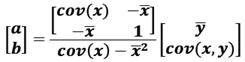
If the data is mean-centered, then a=0 because
For more than one independent variables, say m, we have
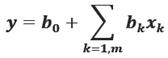
Then we compute b k by minimizing:
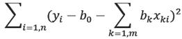
Thus, it determines a hyper-plane which is a least square approximation of data points. If data is mean-centered, then b0=0. It is advised to mean-center data to simplify the computations.
It is interesting to note that as a result of linear regression, the data points may not be at least distance from the regression line. Here we present an algorithm using PCA that results in a better least distance line. There are two ways in which regression analysis is improved: data reduction and hybrid algorithm. As a first step, PCA is used on the dataset for data reduction. For improved performance in the second step, we create a hybrid linear regression algorithm coupled with PCA.
Example: We have a dataset of randomly created 20 points. Matlab computes the regression line as the red line, see Figure 4. PCA computes the blue line. As can be visually seen, the blue line is the least distance line instead of the red regression line. For direction vectors and approximation error of data points from the line, see Table 4.
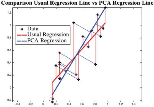
Fig. 4 Using the data points "+", traditional linear regression line is shown in red (LSA) and a principal component is shown in blue (PCA). Visually we can see that the points are much closer to blue line than to the red line.

Both linear regression and PCA compute vectors so that the variation of observed points from the computed vector is minimum. However, as shown in Figure 4, they give two different vectors, red via linear regression, and blue via PCA. The approximation error indicates the PCA adapted regression line is a better approach than by LSA method.
Data reduction is attributed to the non-zero eigenvalues of the data matrix A. Since m x n data matrix is decomposed into A = USVT where U is m x m, S is m x n, and V is n x n. If there are only k non-zero eigenvalues where k ≤ min(m, n), the matrix A has lossless representation by using only k columns of U, k columns of V and kxk diagonal matrix S. If an eigenvalue is very small as compared to others, then ignoring it can lead to further data reduction while retaining most of the information.
B. PCA and Logistic Regression
Along with linear regression, logistic regression (log linear) has been a popular data mining technique. However, both when used stand alone, have limited ability to deal with inter dependent factors. Linear regression is suitable for data that exhibits linear relation, but as all data does not have linear trend, the Logistic models estimate the probability and is applicable to "S-shaped" data. This model is particularly suitable for population growth with limiting condition. As it was with linear regression, it is beneficial to use logistic regression when coupled with PCA.
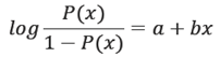
Population growth is described by exponential function; population is controlled by the limiting condition. The liver disease model is a composition of these two functions as shown below. The mapping from linear to logistic function is described as follows [23].
Thus for logistic function P(x) ∈ (0, 1) instead of linear function P(x) = a + bx, the function becomes:

To solve for a and b, we write:
We make use of PCA in designing better logistic regression algorithm, presented below. Here the hybrid algorithm is presented for two-dimensional data, however, it can be easily extended to higher dimensions.

Example: In this example, we have a training dataset of 20 students obtained from [24] who studied for the exam for given hours (horizontal axis) and passed or failed (vertical axis) the test. The curves are the trained logistic regression predictor for chances of passing the exam. Fail and pass are coded numerically as 0 and 1, see Figure 5.
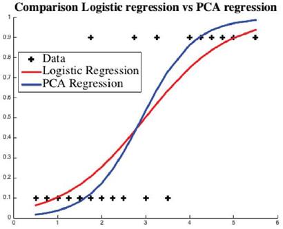
Fig. 5 Using the data points "+", usual logistic regression curve is given in red and the regression curve generated by the proposed hybrid model is given in blue.
The approximation errors for are shown in Table 5. The example exhibits that the PCA (blue) curve is a better approximation predictor with 60% less approximation error.

C. How do we measure the goodness of a model?
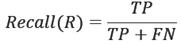
In data mining there are standard measures, called gold standard, for labeling and measuring the prediction accuracy. These measures are useful in comparing the results of classification. Here we will list three metrics, Precision (P), Recall (R) and F-1. In these metrics, actual value and predicted value are used to create a label for each instance outcome, where the instance outcome is either positive or negative. The labels used here are True Positive (TP), False Positive (FP) and False Negative (FN) to measure the accuracy (the reader is encouraged to consult [17] for further details). After labeling, we define the Precision (P), Recall (R) and F-metrics to measure the effectiveness of the prediction on (1) correct prediction on all positive instances and (2) TP prediction on a sample of instances (positive and negative) under investigation on the training data.

The measure F-1 is the weighted Harmonic average of P and R. It is the reciprocal of the weighted average of the reciprocals of P and R.
For 0 ≤ α ≤ 1, it simplifies to:

For α = 0, it turns out to be the recall measure R, for α = 1, it becomes precision measure P, and for α = 1/2, it further simplifies to traditional measure


This is the preferred measure when there are fewer misses of both positive and negative instances, (i.e. both FN and FP are small) [17].
Goodness of fit is an interesting analysis criterion. our goal is to show how the hybrid linear/logistic regression model is better than the more straightforward measures generated for linear/logistic measures.
V. Dimensionality reduction using PCA
The nature of data dictates how many dimensions can be reduced. The data is not just the attributes, but the dependency and redundancy among the attributes. If A=USVT is full dimension SVD of A, where A is m x n, U is m x m, V is n x n, S is m x n, then the total size for decomposition representation of A is m x m + n x n + m x n, which is larger than m x n, the size of A. our goal is to find an integer k smaller than m and n, and use first k columns of U and first k columns of V and restrict S to first k eigenvalues to show the effect of dimensionality reduction. Since eigenpairs are sorted on descending order of variance, deleting the least variation components do not cause significant error in data [25].
In practice, it is not our intent to reconstruct the original matrix A from reduced USVT but to view the data from a fresh perspective and to use the reduced representation to extract information hidden in the original representation. PCA is used to reduce dimensionality in the new space, not the original space. our purpose to see if we can leverage PCA to reduce dimensionality in the original space. This is an open question.

A. Dimension Reduction in Qualitative Spatial Reasoning
PCA has been used mainly with numerical data. If the data is categorical or logical, then data is first converted to numerical. We will see how PCA has the ability to resolve and isolate spatial-temporal patterns in the data presented in Table 2. We present a new robust PCA enabled method for QSR. Table 2 describes eight topological relations between pairs of spatial objects. The values of entries are true and false. In order to use PCA, we first covert the logical data to numerical data. We use 1 for false and 0 for true, see Table 6. our goal is row dimension reduction. As intersection is a complex operation and also computationally expensive, we want to reduce the number of intersections required. For example, for 1000 pairs of objects, there will be 9000 pairwise intersections. By eliminating one intersection, we can reduce 9000 to 8000 intersections, almost 11% improvement in execution. We will show that PCA gives insights, using which we can do better. In fact, we are able to reduce 9000 to 4000 intersections. This is more than 55% reduction in computation time! This means we can replace 9-Intersection model by 4-Intersection model which is now applicable to spatial as well as non-spatial objects, like web documents.
For RCC8, the item-attribute-concept becomes object pair--9-Intersection-relation classification. In Table 6, row header represents a pair of spatial objects, column headers are the 9-Intersection attributes, and last column RCC8 is the classification of the relation based on the intersections. Table 2 and Table 6 show a sample of eight pairs of objects, one of each classification type.
We consider Table 6 is an 8 x 9 input matrix A. on using Matlab SVD on ATA we get nine eigenvectors and nine eigenvalues of ATA shown in Table 7. Since five eigenvalues are zero, the corresponding eigenvectors are useless. This tells us that nx9 data can be replaced with nx4 right away without any loss of information.
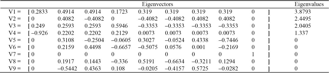
In Table 8, first row enumerates the eigenvalues of
ATA The next rows represent the error on using
first k eigenpairs (where k is the column
number). newA is USVT
based on k eigenpairs used. Error Original is the
|A-newA|/|A| percentage error in the
original space. Error Projection is the |AV-newAV|/|AV|
percentage error in the projection space. Error Eigenvalue is the
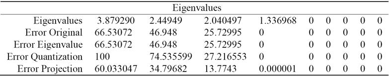
Table 8 shows that the transformed space created using 4 eigenvalues retains perfect information. This means that for all object pairs, the relations can be described with 4 eigenvectors as an n x 4 matrix instead of nx9 matrix with zero error. So how can we deduce the original dimensions that retain most of the information? We explore that in the next section.
VI. Experiments and outcomes
Here we show the application of PCA for dimension reduction in qualitative spatial reasoning and liver disease data. In addition decision tree is used for spatial data classification whereas the improved logistic regression is applied to liver disease data classification.
A. Qualitative Spatial Reasoning
In Section IV, we determined that 4 attributes are sufficient to classify QSR relations in the transformed space. However, it does not tell anything about the attributes in the original space. Now we will see if we can translate this new found knowledge into the original space of Table 2. How can we find four intersection attributes that will lead to the 8 distinct topological relations?
From careful observation of Table 2 we see that the IntInt and BndBnd columns have the most useful information in the sense that they are sufficient to partition the RCC8 relations into eight jointly exhaustive and pairwise distinct (JEPD) classes, which can be further grouped into three classes: {DC, EC}, {NTTP, NTTPc}, and {EQ, TPP, TPPc, PO}.
We revisit Table 2 as Table 9 by shading some entries and analyze them. It shows that only 4-intersections are sufficient for classification of topological relations. The nature of data suggests that the remaining attributes are not necessary. This table can be interpreted and formulated in terms of rules for system integration. These rules are shaded and displayed for visualization in the form of Table 9.
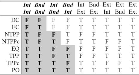
Thus, Table 9 reveals that the spatial relations can be specified by at most four intersection attributes. The shaded columns of Table 9 are transcribed into a decision tree for easy visualization of the rules to classify the RCC8 eight relations, see Figure 6.
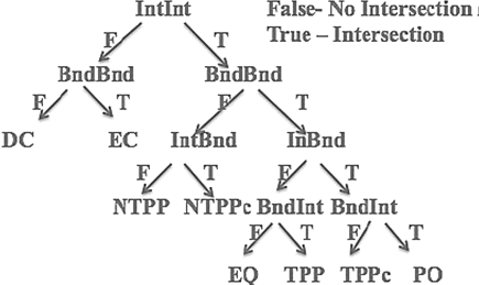
Fig. 6 Classification tree for the topological relations, where T and F represent whether the objects intersect or not respectively.
This conclusion makes no assumptions about the objects being spatial or non-spatial as long as they are valid. In addition, this analysis is applicable to discrete and continuous objects alike.
B. Health Informatics
We will use public domain dataset from uCI Machine Learning Repository [22] to automate the simplicity, applicability and usability of our approach.
For application of our algorithm, we selected liver disease classification dataset. This dataset was selected particularly as most of its attribute were numeric and classification attribute is binary representing presence or absence of the disease. This dataset is compatible with logistic regression and is also well suited to PCA that processes numerical values only.
We obtained the dataset from Machine Learning Repository at the university of California, Irvine [22]. The dataset contains liver disease information about 583 patients out of which 416 are with liver disease and 167 are healthy. The dataset consists of 441 male and 142 female patients. The liver disease classification is based on 10 parameters: age of the patient, gender of the patient, total Bilirubin, direct Bilirubin, Alkaline Phosphotase, Alamine Aminotransferase, Aspartate Aminotransferase, total Proteins, Albumin, Albumin and Globulin ratio. There were two types of recommendations based on these experiments: patient has liver disease or patient does not have liver disease.
This is a fairly small size dataset for classification of 583 patients. Learning from this dataset can be used to predict possible disease for a new patient quickly without further analysis. The goal is not data mining per se, but to show the feasibility of improved algorithms over the existing algorithms and data reduction to classify liver disease. The reduction in one attribute reduces the data size by 9%. We applied PCA on the data to reduce 10 attributes to 3 or 4 attributes, which contribute the most to the eigenvector corresponding to the highest eigenvalue, while retaining approximately the same predictive power as the original data.
For experiment, we created two versions of the dataset: first dataset is raw, the second dataset is mean-centered with unit standard deviation. PCA determines that there is only one non-zero eigenvalue all other eigenvalues are insignificant. one non-zero eigenvalue is shown in Table 10.
This indicates that only a single attribute in the transformed space is sufficient to diagnose the patients. But this does not tell us which original attributes contributed to reduction. The principal components on normalized data are more realistic in this case, as the normalized data attributes values are evenly distributed. For nominal attributes, mapping nominal to numerical can make a difference. However, covariance and correlation approaches are complementary.
The principal component corresponding to non-zero eigenvalue is a linear combination of original attributes. Each coefficient in it is a contribution of the original data attributes. How do we select the fractions of original attributes because the coefficients in this vector are real?
The only thing it means is that each coefficient is a fractional contribution of the original data attributes. It is clear that the three (Alkaline Phosphatase Alamine Aminotransfe-rase, Total Proteins, Aspartate Aminotransferase) of the ten coefficients are more dominant than the others, however normalized data analysis found three more slightly less dominant coefficients. In either case, the contribution of the original three attributes is more than 95%. Eliminating the other attributes, we compute the approximation error due to dimension reduction to three attributes.
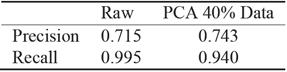
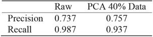
PCA analysis shows that even after 60% reduction, using only 40% of data, the precision is almost the same whereas the gain in computation performance is significant, see Figure 7. For recall, the reduced data regression misses more negatives see Table 11. It is preferable to miss less positive than more negatives. Table 11 corresponds to traditional logistic regression Table 12 corresponds to hybrid logistic regression algorithm. It shows that hybrid algorithm consistently outperforms the traditional algorithms.
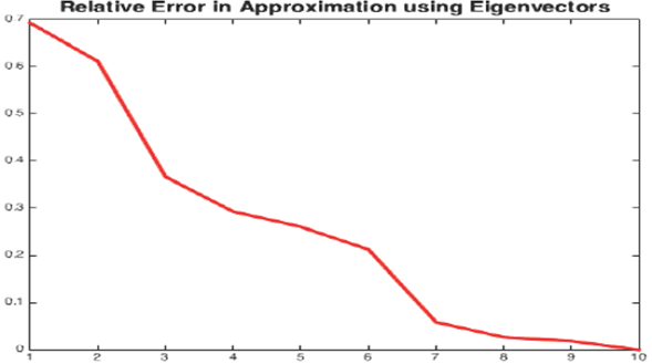
Fig. 7 Error in estimating the original data from eigenvectors where x-axis represents the number of eigenvectors used in data approximation (starting from the most significant to the least significant one) and y-axis represents the error percentage of the estimation.
VII. Conclusion
Principal components analysis is a procedure for identifying a smaller number of uncorrelated variables, called "principal components", from a large set of data. The goal of principal components analysis is to explain the maximum amount of variance with the fewest number of principal components.
Principal components analysis is commonly used as one step in a series of analyses. We use principal components analysis to reduce the number of variables and avoid multi-collinearity, or when we have too many predictors relative to the number of observations. We have used PCA in two diverse genres, QSR and Health Informatics to improve traditional data reduction and regression algorithms.
QSR uses 9-Intersection model to determine topological relations between spatial objects. In general, PCA utilizes numerical data for analysis and as QSR data is logical bivalent, we mapped the logical data to numerical data. PCA determined that 4-attributes are adequate in the transformed space. In general, reduction in transformed space does not tell anything about reduction in base space. However, in this case study, we leveraged PCA to determine the possibility of reduction in the base space. We succeeded in achieving similar reduction the original space of RCC8 relations. This yields more than 55% efficiency in execution time.
We also presented hybrid algorithms that adaptively used PCA to improve the linear and logistic regression algorithms. With experiments, we have shown the effectiveness of the enhancements. All data mining applications that dwell on these two algorithms will benefit extensively from our enhanced algorithms, as they are more realistic than the traditional algorithms. The tables in the paper body vouch for this improvement. We applied our algorithms to the Liver Patient dataset to demonstrate the usability and applicability of our approach, especially in the area of health related data.

