


 text new page (beta)
 English (pdf)
 Article in xml format
 Article references
 Send this article by e-mail
 Cited by SciELO
  Similars in
SciELO
Similars in
SciELO 
 Permalink
I. Introduction
RANDOM networks are a class of complex networks in which there could be link between any two nodes in the network. The Erdos-Renyi (ER) model [1] is a commonly used theoretical model for generating random networks. The ER model-based random networks are characteristic of exhibiting a Poisson-style [2] degree sequence such that the degree of any vertex is typically very close to the average degree of the vertices in the network (i.e., the variation in node degree is typically low). However, the degree sequence of most of the real-world networks rarely follows a Poisson-style distribution; there usually exists an appreciable amount of variation in node degree [3] and there could also be preferential attachment with selected nodes rather than arbitrary attachment [4], Figure 1 shows the degree sequence of the well-known real-world networks with N nodes and L edges and the corresponding ER model-based random networks generated with a probability of link value of 2L/{N(N-1)} [5]. Due to the inherent differences in the nature of the degree sequence, the values for several node-level metrics and network-level metrics exhibited by a ER model-based random network with a certain number of nodes and edges are likely to be independent (correlation coefficient is close to 0) to that of the metric values exhibited by a real-world network with the same number of nodes and edges [5].
Fig. 1 Degree Sequence of Real-World Networks and the Erdos-Renyi (ER) Model-based Random Networks with the Same Number of Nodes and Edges.
In this research, we explore whether a random network whose degree sequence matches to that of a real-world network could exhibit similar values for several critical node-level and network-level metrics as that of the real-world network. In this pursuit, we chose to use the well-known Configuration Model [6] that takes as input the degree sequence of the vertices in any known network and generates a random network with a similar degree sequence. As can be seen in Section 5 of this paper, the correlation coefficient between the degrees of the vertices in the real-world network and the corresponding random network (generated using the Configuration Model) is 0.99 or above. We use a suite of seven node-level metrics and three network-level metrics to evaluate the similarity of each of the real-world network graphs and the corresponding Configuration Model-based random network graphs.
The node-level metrics analyzed are: Degree Centrality, Eigenvector Centrality [7], Betweenness Centrality [8], Closeness Centrality [9], Local Clustering Coefficient [10], Communicability [11] and Maximal Clique Size [12]; the network-level metrics analyzed are: Spectral Radius Ratio for Node Degree [3], Assortativity Index [13] and Algebraic Connectivity [5]. We use a total of 24 real-world network graphs (with different levels of variation in node degree) for this study. We run the appropriate algorithms to determine the individual node-level and network-level metrics on both the real-world graphs and the corresponding random graphs with identical degree sequence. We identify the levels of correlation based on the correlation coefficient values observed for each node-level metric in each of the real-world network graphs and their corresponding Configuration Model-based random network graphs as well as based on the percentage relative difference between the values for each network-level metric for the two graphs.
The rest of the paper is organized as follows: In Section 2, we review the Configuration Model for generating random networks and present a pseudo code for the implementation of the same. In Section 3, we introduce the node-level and network-level metrics evaluated in this paper and briefly describe the appropriate procedures to determine each of them. Section 4 reviews the Spearman's rank-based correlation measure [14] used in the analysis of the real-world networks. Section 5 introduces the real-world networks studied in this paper and analyzes the results for the levels of correlation for the node-level metrics and network-level metrics obtained on the real-world networks and the corresponding random networks generated using the Configuration Model based on the degree sequence of the real-world networks. Section 6 discusses related work on degree preserving randomization of real-world networks. Section 7 concludes the paper and outlines plans for future work. Throughout the paper, we use the terms 'node' and 'vertex', 'link' and 'edge', 'network' and 'graph' interchangeably. They mean the same.
II. Configuration Model
The Configuration Model [6] is one of the well-known models for generating random networks. Its unique characteristic is to take the degree sequence of a given network as input and generate a random network that has the same degree sequence as that of the input network. The degree sequence input to the model need not be Poisson-style - the typical pattern of degree sequence of vertices in random networks generated according to the well-known Erdos-Renyi (ER) model [1]. Thus, the Configuration Model could be used to generate random networks whose degree sequence could correspond to any network of analytical interest. In this paper, we use the Configuration Model to generate random networks whose degree sequence matches to that of real-world networks and we further evaluate the values of the node-level metrics and network-level metrics on both these networks. We are interested in exploring whether a random network whose degree sequence resembles to that of a real-world network exhibits similar values for other critical node-level and network-level metrics.
We simulate the generation of a random network under the Configuration Model as follows. Let N and L be respectively the total number of nodes and edges in a chosen real-world network. Let D be the set of degrees of the vertices (one entry per vertex) in the real-world network. We set up a list L s of vertices - the number of entries for the ID of a vertex in this list is the degree of the vertex in the input set D. After the list L s is constructed, we shuffle the entries in the list. We do the shuffling from the end of the list. In each iteration of shuffling, the ID of a vertex in a particular entry in the list at index i (|Ls| ≥ i ≥ 2) is swapped with the ID of a vertex in a randomly chosen entry at index j (j < i). We now generate the adjacency matrix A conf (each entry is initialized to zero) for the configured graph as follows. We consider the vertex IDs from the end of the shuffled list Ls. For each vertex uID at index u (|Ls| ≥ u ≥ 2) considered, we attempt to pair it with a vertex vID at index v (v < u) such that A cont[uID][vID] = 0 and uID is not the same as vID as well as make sure the entry at index v has not been already paired with another vertex. To keep track of the latter, we set the entries of the shuffled list L s to -1 if the entry is already considered either as an uID or a vID. If a pair (uID, vID) meets the above criteria, we set the entries A cont[uID][vID] = 1 and A cont[uID][vID] = 1. We proceed the iterations until the index u equals 1; by this time, all entries in the shuffled list L s should have been set to -1.
The above implementation procedure for the Configuration model does not generate any self-loop or duplicate edge, as we make sure we are not pairing a vertex with a particular ID at an index u to a vertex with the same ID at another index v as well as we keep track of the edges that have been already configured across all the iterations. To test whether a pair (uID, vID) already have an edge between them, we have to just check the entries for uID or vID in A conf. Thus, each iteration (lines 9-17) is likely to take at most o(N) attempts before a link (uID, vID) is configured. The total number of iterations involving lines 5-8 and lines 9-17 is the sum of the degrees of the vertices in the chosen real-world network. Note that the sum of the degrees of the vertices in a graph is equal to 2L/N where L is the number of links and N is the number of nodes. Hence, the overall time-complexity of the implementation of the Configuration Model described in Figure 2 is O(N x 2L/N) = O(L).

Fig. 2 Pseudo Code for the Implementation of the Configuration Model to Generate Random Graph according to a given Degree sequence.
Figure 3 presents an example to illustrate the generation of a random graph that has the same degree sequence as that of an input graph. The example walks through the sequence of iterations illustrating the execution of the pseudo code given in Figure 2.
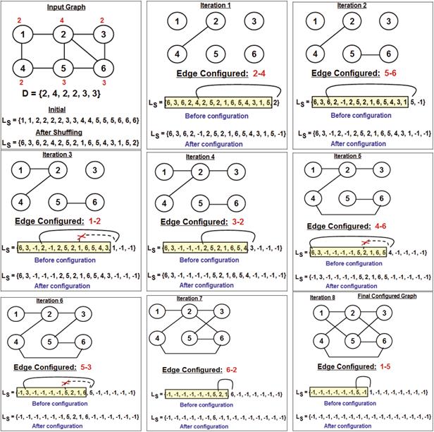
Fig. 3 Example Execution of the Implementation of the Configuration Model to Generate Random Graph according to a given Degree sequence.
We show the contents of the list Ls at the time of initialization (before and after shuffling) as well as during each iteration (before and after the configuration of an edge).
Whenever a vertex pair is picked up for configuring an edge, we replace their entries with -1. We also show sample scenarios wherein we reject the choice of a vID if it is same as that of the uID (shown with a X in iterations 3 and 6) as well as show a sample scenario wherein we reject the choice of a vID (shown with a X in iteration 5) to avoid adding a duplicate edge for the pair (uID, vID). The final configured graph has exactly 8 edges and degree sequence as that of the input graph. However, the edges in the input graph do not match to that of the edges in the final configured graph. As a result, it is not clear whether several other node-level metrics (like the centrality measures, clustering coefficient, communicability, etc.) and network-level metrics (like edge assortativity, algebraic connectivity) would be the same for the two graphs. This is the motivation for the research conducted in the rest of the paper.
III. Node-Level Metrics and Network-Level Metrics
Our objective in this paper is to identify the node-level metrics and network-level metrics for which the degree sequence would be sufficient to observe a very strong correlation between a chosen real-world network graph and its corresponding configuration model generated random network graph. In this pursuit, we study the following node-level metrics (eigenvector centrality, closeness centrality, betweenness centrality, local clustering coefficient, communicability and maximal clique size) and network-level metrics (spectral radius ratio for node degree, edge assortativity and algebraic connectivity).
A. Eigenvector Centrality
The eigenvector centrality (EVC) of a vertex is a measure of the degree of the vertex as well as the degree of its neighbors. The EVC of the vertices in a graph is obtained by computing the principal eigenvector of the adjacency matrix (A) of the graph. In this paper, we use the Power-Iteration algorithm [15] to determine the principal eigenvector/EVC of the vertices. This algorithm is briefly explained as follows.
We start with a unit-column vector of all 1s X0 = [1 1 1 1 ... 1] as the estimated principal eigenvector of the graph where the number of 1s is the number of vertices in the graph. In the (i+1)th iteration, the principal eigenvector Xi+1= AX i / ||AX i || where ||...|| is the normalized value of the product vector obtained by multiplying the adjacency matrix A and the column vector X i.
We continue the iterations until the normalized value of the product vector (as indicated above) does not change beyond a certain level of precision for subsequent iterations. There exists an entry for each of the vertices in the principal eigenvector and the values in these entries correspond to the EVC of the vertices.
Figure 4 illustrates an example to compute the eigenvector centrality of the vertices in a graph using the Power-iteration algorithm. We stop when the normalized value (in the example, it is 2.85) of the product of the adjacency matrix and the principal eigenvector converges and does not change beyond the second decimal. vertex 2 has the highest EVC followed by vertex 6. We notice that though the three vertices 1, 3 and 4 have the same degree, they differ in their EVC values: Both the neighbors of vertex 3 are vertices with higher EVC - as a result, the EVC of vertex 3 is relatively higher than that of vertices 1 and 4. vertex 1 has a higher EVC than vertex 4 (vertices 1 and 4 are also connected to each other) because vertex 1 is connected to a vertex with a higher EVC (vertex 2) while vertex 4 is connected to a vertex (vertex 5) with a relatively lower EVC.

B. Closeness Centrality
The closeness centrality (ClC) [9] of a vertex is the inverse of the sum of the shortest path distances (number of hops) from the vertex to the rest of the vertices in the graph. The ClC of a vertex is determined by running the Breadth First Search (BFS) algorithm [16] on the vertex and determining a shortest path tree rooted at the vertex. one can then easily determine the sum of the number of hops from the vertex to the other vertices in the shortest path tree and the closeness centrality of the vertex is the inverse of this sum. Figure 5 illustrates an example to compute the closeness centrality of the vertices in a graph. We show the shortest path trees rooted at each vertex and compute the number of hops from the root to the rest of the vertices in these trees to arrive at the distance matrix, contributing to the computation of the closeness centrality.

C. Betweenness Centrality
The betweenness centrality (BWC) [8] of a vertex is a measure of the fraction of the shortest paths between any two vertices that go through the particular vertex, summed over all pairs of vertices. The number of hops for a vertex from the root of a shortest path tree indicates the level of the vertex on the tree. The number of shortest paths, denoted sp jk, from a vertex j to a vertex k at level l (l > 0) is the sum of the number of shortest paths from j to each of the neighbors of k (in the original graph) that are at level l -1 in the shortest path tree rooted at j. For any vertex i, the number of shortest paths from vertex j to vertex k that go through i, denoted sp jk(i), is the maximum of the number of shortest paths from vertex j to vertex i and the number of shortest paths from vertex k to vertex i. Quantitatively, the BWC of a vertex i is defined as

Figure 6 shows an example illustrating the computation of the BWC of the vertices in a graph.

D. Local Clustering Coefficient
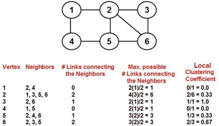
The local clustering coefficient (LCC) [10] of a vertex in a graph is a measure of the probability that any two neighbors of the vertex are connected. Quantitatively, the local clustering coefficient of a vertex is the ratio of the actual number of links between the neighbors of the vertex divided by the maximum possible number of links between the neighbors of the vertex. For a vertex i with degree ki, if there are a total of l links connecting the neighbors of i, then the clustering coefficient of i is

Figure 7 shows an example of computing the local clustering coefficient of the vertices of a graph.
E. Communicability
The communicability (COMM) [11] of a vertex is the weighted sum of the number of walks of lengths l = 1, 2, 3,... from that vertex to each of the other vertices in the graph, with the weight being 1/!. A walk from vertex r to s involves a sequence of intermediate vertices that may or may not appear more than once. That is, a walk could involve cycles. The communicability of a vertex captures the ease with which a vertex can disseminate information to the rest of the vertices through various walks (the shortest paths are given more weights though). Though the definition of the communicability of a vertex could be represented mathematically as in equation (1), we use the closed form equation (2) to quantitatively determine the communicability of the vertices in a graph [11]. (Al) rs represents the number of walks of length l between two vertices r and s. Note that for a graph of n vertices (where V is the set of vertices, |V| = n), there are n eigenvalues (denoted as λ j where j = 1, 2,...n) and the corresponding eigenvectors (denoted as ϕj, where j = 1, 2,..., n). ϕj (r) and ϕj(s) denotes the values for vertices r and s in the eigenvector associated with eigenvalue λ j. We compute the eigenvalues and eigenvectors of the adjacency matrix of a graph using the JAMA package [17].
 (1)
(1)
 (2)
(2)
F. Maximal Clique Size
A clique is a subset of the vertices of a graph such that there exists an edge between any two vertices in this set. Each vertex in a graph is part of at least one clique, as even an edge could be considered a clique of size 2. We refer to the maximal clique for a vertex as the largest size clique that the vertex is part of and call the size of the corresponding clique as the maximal clique size [12]. We refer to the maximum clique size of the entire graph as the largest of the maximal clique size (MCS) values of the vertices [18]. As observed in the example shown in Figure 9, one or more vertices (vertices 4, 5, 6, 7) could be part of a maximum clique size, while for the rest of the vertices (vertices 1, 2 and 3), the maximal clique size could be less than maximum clique size. We use the extended version of an exact algorithm by Pattabiraman et al [18] to determine the maximal clique size for each vertex. The algorithm takes a branch and bound approach of exploring all possible candidate cliques that a vertex could be part of, but searching through only viable candidate sets of vertices whose agglomeration has scope of being a clique of size larger than the currently known clique found as part of the search.


Figure 8 presents the communicability of the vertices for the same example graph (of six vertices) used in Figures 4, 5 and 7. The figure also lists the six eigenvalues and the corresponding eigenvectors that are used in the calculations of the communicability of the vertices (according to equation 2). We observe vertex 2, followed by vertex 6, to have the largest values for communicability. In general, vertices having a higher degree and part of a closely-knit community (vertices 2, 3, 5 and 6 would have formed a clique had there been an edge 3-5). Notice that between vertices 5 and 6 (both of which have degree 3), vertex 6 has a slightly larger communicability, attributed to the connection of vertex 6 to vertex 3 that is in turn connected to vertex 2 (whereas vertex 5 is connected to vertex 4 that is not connected to vertex 2, but instead connected to a low-degree vertex, vertex 1). Likewise, between vertices 1, 3 and 4 (all of which have degree 2), vertex 3 has the highest communicability as it is connected to vertices 2 and 6 - both of which have a high communicability.
G. Spectral Radius Ratio for Node Degree
The spectral radius of a graph G, denoted λsp(G), is the principal eigenvalue (largest eigenvalue) of the adjacency matrix of the graph. If k min, kavg and k max are the minimum, average and maximum node degrees, then k mim ≤ kavg ≤ λsp(G) ≤ k max [19]. As one can see from this relationship, the spectral radius could be construed as a measure of the variation in the degree of the vertices in a graph. In [3], the notion of spectral radius ratio for node degree was proposed to evaluate the variation in node degree on a uniform scale, without the need for explicitly computing the variance/standard deviation of the vertices in the graph. The spectral radius ratio for node degree is the ratio of the spectral radius of the graph and the average degree of the vertices in the graph: λsp(G)/kavg. According to the above formulation, the spectral radius ratio for node degree values are always 1.0 or above; the farther the value is from 1.0, the larger the variation in node degree among the vertices of the graph. Figure 10 presents an example to illustrate the relationship k mim ≤ kavg ≤ λsp(G) ≤ k max and the spectral radius ratio for node degree. As this ratio is closer to 1.0, we could construe that the variation in node degree is very less; we can see 50% (three out of six) of the vertices have degree 2 and one-third (two out of six) of the vertices have degree 3, leading to an average degree of 2.67.

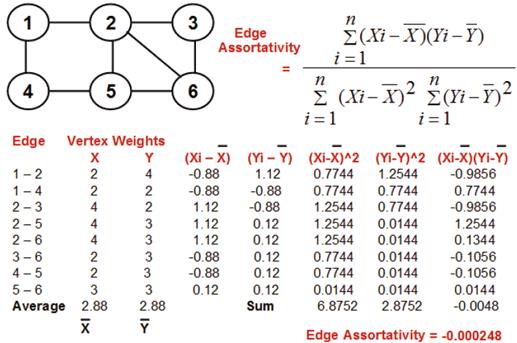
H. Edge Assortativity
The assortativity of the edges in a graph is a measure of the similarity of the end vertices of the edges based on any notion of node weights [13]. In this research, we use node degree as the measure of node weight. Quantitatively, edge assortativity is essentially the correlation coefficient of the node weights of the end vertices. If the correlation coefficient is close to 1.0, - 1. 0 and 0.0 respectively, we could say the end vertices of the edges are respectively maximally similar, maximally different and independent to each other based on the notion of node weights considered. Figure 11 presents an example to calculate edge assortativity in a graph, wherein the ids of the vertices constituting an edge are considered as an ordered pair (i, j) such that i < j. We observe the correlation coefficient (edge assortativity) to be close to 0.0, indicating that the pairing of the vertices that constitute the edges of the graph is independent of the degrees of the end vertices constituting these edges. ER model-based Random graphs [1] exhibit an edge assortativity close to 0 indicating the arbitrary pairing of the vertices to constitute the edges.
I. Algebraic Connectivity
The algebraic connectivity of a graph is a quantitative measure of the connectivity of the graph capturing the vulnerability of a graph for disconnection as a function of the number of vertices in the graph as well as the topology of the graph [20]. The algebraic connectivity of a graph is bounded above by the traditional connectivity of the graph, defined as the minimum number of vertices that need to be removed to disconnect the graph into two or more components [21]. However, the traditional connectivity measure (an integer corresponding to the minimum number of vertices to be removed for disconnection) cannot capture the relative strength of the graph with respect to node removals. For two graphs having the same value of traditional connectivity, the algebraic connectivity could be still different [21]. The larger the value of the algebraic connectivity, the stronger the graph - only the removal of certain nodes could disconnect the graph (and not the removal of any node).
Quantitatively, for a connected graph, the algebraic connectivity is measured to be the second smallest eigenvalue of the Laplacian Matrix (L) of a graph [22]. In addition, for a connected graph, the smallest eigenvalue of the Laplacian Matrix of the graph is always 0. In general, the number of zeros among the eigenvalues of the Laplacian Matrix of a graph indicates the number of connected components of the graph [23]. The entries in the Laplacian Matrix of a graph are defined as follows [23]:
L(i, j) = degree(i) if i = j
= -1 for i ≠ j and edge (i, j) exists
= 0 for i ≠ j and edge (i, j) does not exist
Figure 12 presents examples to determine the Laplacian Matrices of two graphs and compute the sequence of eigenvalues for the two matrices. There is only one zero among the eigenvalues of the Laplacian matrices of both the graphs, indicating that both the graphs are connected and all the vertices form a single connected component. Graph-2 is relatively stronger than Graph-1 due to the presence of an additional edge 2-4 in the former.

Fig. 12 Example to Illustrate the Determination of Algebraic Connectivity and its Use a Measure of Evaluation of the Relative Strengths of Two Graphs with the Same Traditional Connectivity.
Though both the graphs have a traditional connectivity of 2 (both the graphs get disconnected with the removal of vertices 2 and 5 in each of them), the removal of any two vertices from the graph is relatively more likely to lead to a disconnection in Graph-1 compared to Graph-2. One could notice that the removal of vertices 1 and 5 could disconnect vertex 4 from the rest of the vertices in Graph-1; on the other hand, the removal of vertices 1 and 5 would not disconnect vertex 4 from the rest of the vertices in Graph-2.
IV. Spearman's Rank-Based Correlation Measure
We resort to a rank-based correlation coefficient study in this paper as we want to explore the level of similarity between the ranking of the vertices (with respect to a node-level metric) in a real-world network graph and the corresponding degree-preserved random network graph. In this pursuit, we choose to use the Spearman's rank-based correlation measure (SCC). SCC is a measure of how well the relationship between two datasets (variables) can be assessed using a monotonic function [14]. To compute the SCC of two datasets (say, A and C), we convert the raw scores Ai and Ci for a vertex i to ranks ai and ci and use formula (3) shown below, where di = ai - ci is the difference between the ranks of vertex i in the two datasets. We follow the convention of assigning the rank values from 1 to n for a graph of n vertices with vertex IDs that are also assumed to range from 1 to n. To obtain the rank for a vertex based on the list of values for a node-level metric, we first sort the values (in ascending order). If there is any tie, we break the tie in favor of the vertex with a lower ID; we will thus be able to arrive at a tentative, but unique, rank value for each vertex with respect to the metric. We determine a final ranking of the vertices as follows: For vertices with unique value of the node-level metric, the final ranking is the same as the tentative ranking. For vertices with an identical value for the node-level metric, the final ranking is assigned to be the average of their tentative rankings. Figure 13 illustrates the computation of the tentative and final ranking of the vertices based on their BWC values in the actual graph and the configuration model-based random network graph generated in Figure 3 as well as illustrates the computation of the Spearman's rank-based correlation coefficient.
 (3)
(3)

Fig. 13 Example to Illustrate the Computation of the Spearman's Rank-based Correlation Coefficient with respect to BWC on the Actual Graph and Configured Graph of Figure 3.
In Figure 13, we observe ties among vertices with respect to BWC in both the actual graph and the corresponding configured graph. The tentative ranking is obtained by breaking the ties in favor of vertices with lower IDs. In the case of the actual graph, we observe both vertices 1 and 6 to have an identical BWC value of 0.83 each and their tentative rankings are respectively 3 and 4 (ties for tentative rankings are broken in favor of vertices with lower IDs); the final ranking (3.5) for both these vertices is thus the average of 3 and 4. A similar scenario could be observed for the configured graph: vertices 1 and 3 have an identical BWC value of 0.33 each and their tentative rankings are respectively 2 and 3; the final ranking (2.5) for both these vertices is thus the average of 2 and 3. The Spearman's rank-based correlation coefficient with respect to BWC for the actual graph and configured graph in Figure 13 is observed to be 0.87, indicating a very strong positive correlation. A ranking of the vertices with respect to BWC in the actual graph is: 3, 4, 1-6 (tie), 5 and 2; whereas the ranking of the vertices with respect to BWC in the configured graph is: 4, 1-3 (tie), 6, 5 and 2.
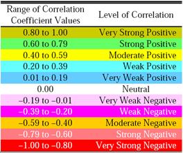
The correlation coefficient values obtained for all the node-level metrics range from -1 to 1. Correlation coefficient values closer to 1 for a node-level metric indicate that identical degree sequence for the real-world network graph and the configuration model based random network graph is sufficient to generate an identical ranking of the vertices in the two graphs with respect to the metric. Correlation coefficient values closer to -1 for a node-level metric indicate that identical degree sequence between the real-world network graph and the configuration model based random network graph is sufficient to generate a ranking of the vertices in the real-world network graph that is the reversal of the ranking of the vertices in the corresponding configuration model-based random network graph (i.e., a highly ranked vertex with respect to the particular node-level metric in the real-world network graph is ranked much low with respect to the same metric in the corresponding random network graph and vice-versa). Correlation coefficient values closer to 0 indicate no correlation (i.e., an identical degree sequence alone is not sufficient to generate an identical ranking of the vertices with respect to the node-level metric in the real-world network graph and the corresponding random network graphs). We will adopt the ranges (rounded to two decimals) proposed by Evans [23] to indicate the various levels of correlation, shown in Table 1. The color code to be used for the various levels of correlation is also shown in this table.
V. Real-World Networks
We analyze a total of 24 real-world networks with different levels of variation in node degree. The spectral radius ratio for node degree (λsp(K)) for these networks varies from 1.04 to 3.0, with the type of networks ranging from random networks to scale-free networks [4]. All networks are modeled as undirected networks. A brief description of the 24 real-world networks (a three-character abbreviation for each of these networks is indicated in the parenthesis), in the increasing order of their spectral radius ratio for node degree, is as follows:
Macaque Dominance Network (MDN) [24]: This is a network of 62 adult female Japanese macaques (monkeys; vertices) in a colony, known as the "Arashiyama B Group", recorded during the non-mating season from April to early October 1976. There exists an edge between two vertices if the one of the two corresponding macaques exhibited dominance over the other macaque.
College Fraternity Network (CFN) [25]: This is a network of 58 residents (vertices) in a fraternity at a West Virginia college; there exists an edge between two vertices if the corresponding residents were seen in a conversation at least once during a five day observation period.
Hypertext 2009 Network (HTN) [26]: This is a network of the face-to-face contacts of 113 attendees (vertices) of the ACM Hypertext 2009 conference held in Turin, Italy from June 29 to July 1, 2009. There exists an edge between two vertices if the corresponding conference visitors had face-to-face contact that was active for at least 20 seconds.
Flying Teams Cadet Network (FTC) [27]: This is a network of 48 cadet pilots (vertices) at an US Army Air Forces flying school in 1943 and the cadets were trained in a two-seated aircraft. There exists an edge between two vertices if at least one of the two corresponding pilots has indicated the other pilot as his/her preferred partner with whom s/he likes to fly during the training schedules.
Sawmill Strike Communication Network (SSC) [28]: This is a network of 24 employees (vertices) in a sawmill who planned a strike against the new compensation package proposed by their management. There exists an edge between any two vertices if the corresponding employees mutually admitted (to an outside consultant) discussing about the strike with a frequency of three or more (on a 5-point scale).
Primary School Contact Network (PSN) [29]: This is a network of children and teachers (vertices) used in the study published by an article in BMC Infectious Diseases, 2014. There exists an edge between two vertices if the corresponding persons were in contact for at least 20 seconds during the observation period.
Mexican Political Elite Network (MPN) [30]: This is a network of 35 Mexican presidents and their close collaborators (vertices); there exists an edge between two vertices if the corresponding two people have ties that could be either political, kinship, friendship or business ties.
Residence Hall Friendship Network (RHF) [31]: This is a network of 217 residents (vertices) living at a residence hall located on the Australian National University campus. There exists an edge between two vertices if the corresponding residents are friends of each other.
UK Faculty Friendship Network (UKF) [32]: This is a network of 81 faculty (vertices) at a UK university. There exists an edge between two vertices if the corresponding faculty are friends of each other.
World Trade Metal Network (WTM) [33]: This is a network of 80 countries (vertices) that are involved in trading miscellaneous metals during the period from 1965 to 1980. There exists an edge between two vertices if one of the two corresponding countries imported miscellaneous metals from the other country.
Jazz Band Network (JBN) [34]: This is a network of 198 Jazz bands (vertices) that recorded between the years 1912 and 1940; there exists an edge between two vertices if the corresponding bands had shared at least one musician in any of their recordings during this period.
Karate Network (KAN) [35]: This is a network of 34 members (nodes) of a Karate Club at a US university in the 1970s; there is an edge between two nodes if the corresponding members were seen interacting with each other during the observation period.
Dutch Literature 1976 Network (DLN) [36]: This is a network of 35 Dutch literary authors and critics (vertices) in 1976. There exists an edge between two vertices if one of them had made a judgment on the literature work of the author corresponding to the other vertex.
Senator Press Release Network (SPN) [37]: This is a network of 92 US senators (vertices) during the period from 2007 to 2010. There exists an edge between two vertices if the corresponding senators had issued at least one joint press release.
ModMath Network (MMN) [38]: This is a network of 38 school superintendents (vertices) in Allegheny County, Pennsylvania, USA during the 1950s and early 1960s. There exists an edge between two vertices if at least one of the two corresponding superintendents has indicated the other person as a friend in a research survey conducted to see which superintendents (who are in office for at least a year) are more influential to effectively spread around some modern Math methods among the school systems in the county.
C. Elegans Neural Network (ENN) [39]: This is a network of 297 neurons (vertices) in the neural network of the hermaphrodite Caenorhabditis Elegans; there is an edge between two vertices if the corresponding neurons interact with each other (in the form of chemical synapses, gap junctions, and neuromuscular junctions).
Word Adjacency Network (WAN) [40]: This is a network of 112 words (adjectives and nouns, represented as vertices) in the novel David Copperfield by Charles Dickens; there exists an edge between two vertices if the corresponding words appeared adjacent to each other at least once in the novel.
Les Miserables Network (LMN) [41]: This is a network of 77 characters (nodes) in the novel Les Miserables; there exists an edge between two nodes if the corresponding characters appeared together in at least one of the chapters in the novel.
Copperfield Network (CFN) [41]: This is a network of 87 characters in the novel David Copperfield by Charles Dickens; there exists an edge between two vertices if the corresponding characters appeared together in at least one scene in the novel.
Graph and Digraph Glossary Network (GLN) [42]: This is a network of 72 terms (vertices) that appeared in the glossary prepared by Bill Cherowitzo on Graph and Digraph; there appeared an edge between two vertices if one of the two corresponding terms were used to explain the meaning of the other term.
Centrality Literature Network (CLN) [43]: This is a network of 129 papers (vertices) published on the topic of centrality in complex networks from 1948 to 1979.
There is an edge between two vertices if one of the two papers has cited the other paper as a reference.
Citation Graph Drawing Network (GDN) [44]: This is a network of 311 papers (vertices) that were published in the Proceedings of the Graph Drawing (GD) conferences from 1994 to 2000 and cited in the papers published in the GD'2001 conference. There is an edge between two vertices if one of the two corresponding papers has cited the other paper as a reference.
Anna Karenina Network (AKN) [41]: This a network of 138 characters (vertices) in the novel Anna Karenina; there exists an edge between two vertices if the corresponding characters have appeared together in at least one scene in the novel.
Erdos Collaboration Network (ERN) [45]: This is a network of 472 authors (nodes) who have either directly published an article with Paul Erdos or through a chain of collaborators leading to Paul Erdos. There is an edge between two nodes if the corresponding authors have co-authored at least one publication.
We generate 100 instances of the configuration model-based random network graphs for each of the real-world network graphs. We compute the following seven node-level metrics on each of the real-world network graphs and the corresponding 100 instances of the random network graphs generated according to the Configuration model:
Degree Centrality,
Eigenvector Centrality,
Closeness Centrality,
Betweenness Centrality,
Clustering Coefficient,
Communicability and
Maximal Clique Size.
For each real-world network, we average the values for each of the above node-level metrics obtained for the 100 instances of the random network graphs with identical degree sequence. For each node-level metric, we then determine the Spearman's rank-based correlation coefficient between the values incurred for the metric in each of the 24 real-world network graphs and the average values for the metric computed based on the 100 instances of the corresponding configuration model-based random network graphs.
Table 2 lists the correlation coefficient values obtained for the seven node-level metrics for each real-world network graph and the corresponding configuration model-based instances of the random network graphs with an identical degree sequence. As expected, the correlation coefficient values for the degree centrality are either 0.99 or 1.0, vindicating identical degree sequence between the two graphs. The Communicability metric exhibits a very strong positive correlation for all the 24 network graphs. With respect to three centrality metrics (EVC, ClC, BWC), we observe a strong-very strong positive correlation for all the 24 network graphs, with the EVC exhibiting very strong positive correlation for 20 of the 24 real-world networks and the ClC and BWC metrics exhibiting very strong positive correlation for 17 and 18 of the 24 real-world networks respectively. The maximal clique size (MCS) metric exhibits strong-very strong positive correlation for 17 of the 24 real-world networks (very strongly positive correlation for 7 real-world networks and strongly positive correlation for 10 real-world networks). The local clustering coefficient (LCC) is the only node-level metric for which we observe a poor correlation between the real-world network graphs and the corresponding random network graphs with identical degree sequence. The level of correlation is very weak to at most moderate for 14 of the 24 real-world networks and very strongly positive for just one real-world network.
Table II Correlation coefficient values for the node-level metrics between the real-world network graphs and the corresponding instances of configuration model-based random network graphs.
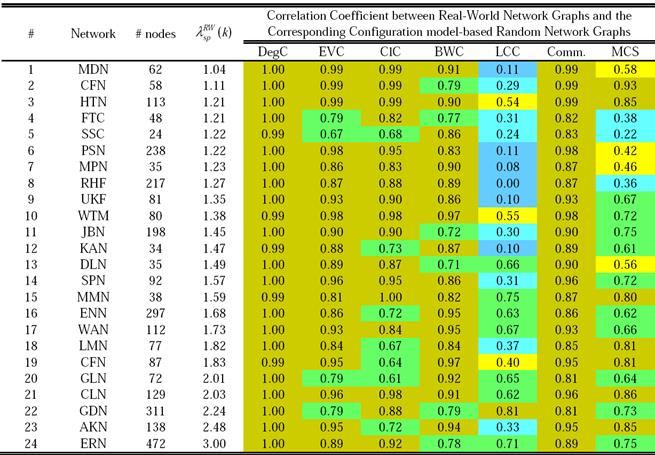
We summarize the above observations on the basis of the percentage chances of finding a real-world network graph with a very strong positive correlation with its corresponding configuration model-based random network graph (with an identical degree sequence) as follows: While there is a 100% chance (24 out of 24 networks) for a very strongly positive correlation in the case of communicability; for the three centrality metrics: the percentage chances of observing a very strongly positive correlation are respectively 83% (20 out of 24 networks) for EVC, 75% (18 out of 24 networks) for BWC and 71% (17 out of 24 networks) for ClC. In the case of maximal clique size and local clustering coefficient, the percentage chances of obtaining a very strong positive correlation are respectively 29% and 4%.
With respect to the impact of the spectral radius ratio for node degree on the correlation levels observed for the node-level metrics (see Figure 14), we observe the correlation levels for communicability and the centrality metrics to be independent of the spectral radius ratio for node degree. The correlation coefficient values for communicability and the centrality metrics (EVC, ClC and BWC) are consistently high (0.6 or above) for all the 24 real-world network graphs, irrespective of the values for the spectral radius ratio for node degree. In the case of both local clustering coefficient and maximal clique size, we observe the correlation levels to increase with increase in the spectral radius ratio for node degree (i.e., as the real-world networks are increasingly scale-free, we observe the correlation levels for these two metrics to increase with that of the configuration model-based random network graphs with identical degree sequence).

Fig. 14 Example to Illustrate the Computation of the Spearman's Rank-based Correlation Coefficient with respect to BWC on the Actual Graph and Configured Graph of Figure 3.
Table 3 lists the values for the three network-level metrics (spectral radius ratio for node degree, degree-based edge assortativity and algebraic connectivity) for the real-world network graphs and the corresponding configuration model-based random network graphs with identical degree sequence.
Table III Comparison of the values for the network-level metrics: real-world network graphs and the configuration model-based random network graphs with identical degree sequence.

The value for a network-level metric reported for the random network graph corresponding to a real-world network graph is the average of the values for the metric evaluated on 100 instances of the random network graphs for the particular real-world network graph. In Table 3, we have colored the cells (in yellow) for which a graph (real-world network graph or the configuration model-based random network graph) incurs an equal or relatively larger value for the network-level metric. Figure 15 illustrates the distribution of the above three network-level metrics for both the real-world network graphs and the corresponding random network graphs. For each network-level metric, we evaluate the proximity of the data points to the diagonal line. The more closer are the data points to the diagonal line, the more closer are the values for the particular network-level metric for both the real-world network graph and the corresponding random network graph.
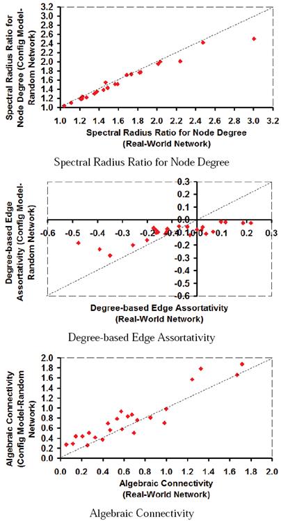
Fig. 15 Distribution of the Values for the Network-Level Metrics for Real-World Network Graphs and the Configuration Model-based Random Network Graphs with Identical Degree sequence.
With respect to the spectral radius ratio for node degree, the general trend of the results is that for more than 20 of the 24 real-world network graphs, the spectral radius ratio for node degree is observed to be just marginally greater than the average value of the spectral radius ratio for node degree of the 100 corresponding instances of the configuration model-based random network graphs with identical degree sequence.
From Figure 14, except of a couple of real-world network graphs, we observe the data points for the spectral radius ratio for node degree to lie closer to the diagonal line, indicating both the real-world network graphs and their corresponding configuration model-based random network graphs incur comparable values for this metric, with the random network graphs consistently incurring slightly lower values for most cases.
With respect to the degree-based edge assortativity, we observe the configuration model-based random network graphs to incur negative values for the degree-based edge assortativity for all the 24 real-world network graphs analyzed (even though the edge assortativity values were positive for 1/3rd of the real-world network graphs). Thus, the configuration model-based random network graphs are highly likely to be dissortative even though their corresponding real-world network graphs are assortative. On the other hand, for real-world network graphs with negative values for the degree-based edge assortativity, we observe the edge assortativity of the corresponding configuration model-based random network graphs to be relatively larger (i.e., farther away from -1). That is, for dissortative real-world network graphs, the corresponding configuration model-based random network graphs are likely to be relatively less dissortative. With respect to connectivity, we claim the configuration model-based random network graphs are more likely to exhibit relatively higher values for algebraic connectivity compared to their corresponding real-world network graphs (as is observed for 16 of the 24 real-world network graphs).
VI. Related Work
Degree preserving randomization [46] has been widely considered a technique of assessing whether the values for the node-level metrics and network-level metrics for a real-world network graph is just an artifact of the graph's inherent structural properties or properties that are unique for the nodes. Monte Carlo-based methods [47] were earlier used to generate random network graphs with identical degree sequence as that of the real-world networks. However, these methods were found to require a significant number of iterations (significantly larger than the number of edges in the real-world graphs) as well as are prone to introducing self-loops and multi-edges. The work in [48] formed the basis for modeling real-world social networks as random network graphs and evaluating the node-level metrics and network level metrics for the two graphs. For certain social networks, network-level metrics such as the global clustering coefficient and the average path length were observed to be closer to that of the equivalent random networks and much different for others. The difference in the values for the network-level metrics is attributed to the sociological structure and influence among nodes not being captured in the random networks even though they are modeled to have an identical degree sequence to that of the social networks [48]. The authors in [49] conclude that global network-level metrics cannot be expected to be even closely reproduced in random network graphs generated with local constraints (such as the degree-preserving randomization). To corroborate this statement, degree-preserved randomized versions of the internet at the level of Ass (As - Autonomous systems) are observed to have a fewer number of k-shells [50]. A k-shell is the largest sub graph of a graph such that the degree of every vertex is at least k within the sub graph [51]. The distribution of the k-shells has been observed to be dependent on the connectivity of the nodes in the network and hence the number of k-shells has been perceived to be a network-level metric [50].
Random networks generated from the traditional ER model have been observed to incur lower values for the local clustering coefficient (proportional to the probability of a link between any two nodes in the ER model) [5]; the correlation coefficient analysis studies in this paper also indicate that the local clustering coefficient of the configuration model-based random network graphs do not correlate well with those of the corresponding real-world network graphs with an identical degree sequence. in [52], the authors proposed random graph models whose local clustering coefficient is as large as those observed for real-world networks as well as generate a power-law degree pattern [4] that could be controlled using certain operating parameters.
In another related study [53], degree-preserved random networks of a certain number of nodes and edges were observed to contain more feed forward loops (FFLs) when compared to the ER-random networks of the same number of nodes and edges; but the number of FFLs in the degree-preserved random networks has been observed to be significantly lower than the corresponding real-world biological networks. Degree preserving randomization was successfully applied in [54] to determine that clustering and modularity do not impact the number of driver nodes needed to effectively control real-world networks. in a related study, it was observed that the degree sequence of a real-world network was alone sufficient to generate a random network whose distribution for the control centrality [55] of a node was identical to that of the real-world network. The control centrality of a node [55] in a directed weighted network graph is a quantitative measure of the ability of a single node to control the entire network.
Even though several such studies have been conducted on degree-preserving randomization of real-world networks and analysis of the resulting random networks, no concrete information is available on the impact of the identical degree sequence on the centrality metrics (as well as the other node-level and network-level metrics considered in this paper such as communicability, maximal clique size, degree-based edge assortativity, algebraic connectivity and spectral radius ratio for node degree) for the real-world social networks and the equivalent degree-preserved random networks. We have to resort to a correlation-based study as the distribution profiles for a node-level metric in the real-world network graph and the corresponding degree-preserved random network graph is not sufficient to study the similarity in the ranking of the vertices in the two graphs with respect to the metric. To the best of our knowledge, ours is the first such study to comprehensively evaluate the similarity in the ranking of the vertices between the real-world network graphs and the corresponding degree-preserved random network graphs with respect to the centrality metrics and maximal clique size as well as to use the Spearman's rank-based correlation measure for correlation study in complex network analysis.
VII. Conclusions and Future Work
The results from Table 2 indicate that the ranking of the vertices in a real-world network graph with respect to the centrality metrics and communicability is more likely to be the same as the ranking of the vertices in a random network graph (generated according to the configuration model with an identical degree sequence) as a very strongly positive correlation (correlation coefficient values of 0.8 or above) is observed for a majority of the real-world networks analyzed. on the other hand, we observe that an identical degree sequence is not sufficient to increase the chances of obtaining an identical ranking of the vertices in a real-world network graph and its corresponding degree-preserved random network graph with respect to maximal clique size and local clustering coefficient. Thus, the maximal clique size and local clustering coefficient are node-level metrics that depend more on the network structure rather than on the degree sequence.
The results from Table 3 indicate that the spectral radius ratio for node degree is likely to be more for a real-world network graph vis-a-vis a random network graph with an identical degree sequence. on the other hand, we observe that all the degree-preserved random network graphs generated according to the configuration model are dissortative irrespective of the nature of assortativity of the corresponding real-world network graphs; nevertheless, the level of dissortativity is relatively less for degree-preserved random network graphs generated for real-world networks that are also dissortative. We observe that a random network graph is more likely to exhibit higher values for algebraic connectivity compared to the real-world network graph with which it has an identical degree sequence. As part of future work, we plan to run the community detection algorithms on the configuration model generated random network graphs and compare the modularity of the communities with those detected in the corresponding real-world network graphs with an identical degree sequence.

