


 nueva página del texto (beta)
 Inglés (pdf)
 Artículo en XML
 Referencias del artículo
 Enviar artículo por email
 Citado por SciELO
  Similares en
SciELO
Similares en
SciELO 
 Permalink
Introduction
Mexico is a large middle-income country debating between progressing to eventually becoming a developed nation or remaining anchored to its historical ballasts such as inequality, poverty, corruption, and crime. Mexico opened its economy, became part of the North American Free Trade Agreement with United States and Canada, and performed several structural reforms in just three decades (e.g., autonomy of the central bank, fiscal discipline), but on the other hand Mexico experiences a proliferation of powerful drug cartels and an upsurge of violence in the last two decades.
Despite the dramatic increase in the incidence of crime in Mexico, research on its economic consequences has been limited. Kato (2013) and Medellín et al. (2015) have addressed the problem using Becker (1968) approach, while Quiroz et al. (2015), Cabrera et al. (2018) have done so using time series econometrics. Even though these studies show the potential of criminal activities to negatively affect investment and economic activity, they related with general crime and violence and not business insecurity in specific. Also, they did not study the fiscal incidence of crime once it is modeled as a tax on business activities.
This article contributes to the literature on the economic consequences of crime among businesses in Mexico. This is accomplished by introducing crime as a combination of sales or capital use taxes into a static general equilibrium model of the Mexican economy that was built from a social accounting matrix. Within this framework, it is possible to assess the magnitude of the economic losses of business insecurity as proportion of the GDP, as well as to make the fiscal incidence analysis of the crime tax among households and firms under different scenarios.
Antecedents: The recent upsurge of crime in Mexico
There is evidence of a recent hike in criminal activity in Mexico. There are many ways to measure this. The most common way to measure crime is with the homicide rate which measures the number of homicides for every 100,000 inhabitants. Figure 1 presents the evidence of homicides over Mexico’s last three decades. The results illustrate that the homicide rate steadily decreased between 1990 and 2007; it was more than cut in half, from 18 to 8 homicides for every 100,000 inhabitants. In 2008, the decreasing trend was broken, as the homicide rate began growing annually at a rapid pace. It exceeded 20 homicides between 2011 and 2012. The rate reached a new maximum of 29 homicides for every 100,000 inhabitants recently.
Source: Instituto Nacional de Estadística y Geografía (INEGI).
Figure 1 Mexico’s Homicide rate (Total homicides per every 100, 000 inhabitants)
The sustained increase in violent crime in Mexico is not a common trend among typical middle and high-income nations. According to the latest violence figures provided by the United Nations Office of Drugs and Crime (UNODC), Mexico’s homicide rate of 29 homicide victims per 100,000 people is the highest among the countries listed in Table 1. This rate is comparable to that of Brazil and Colombia and is well above that of the United States and Canada, Mexico’s main trading partners. Even though Colombia’s rate is currently at the 25 level, it has decreased significantly since the nineties, unlike Mexico’s increase.
Table 1 Homicide rate among middle and high-income countries (Total homicides per every 100, 000 inhabitants)
| 1990 | 1994 | 2000 | 2006 | 2012 | 2018 | |
|---|---|---|---|---|---|---|
| Mexico | 17.3 | 17.6 | 10.9 | 9.7 | 22.1 | 29.1 |
| Brazil | 19.7 | 18.7 | 23.8 | 24 | 26.6 | 27.4 |
| Colombia | 73.5 | 75.7 | 67 | 40.5 | 35.7 | 25.3 |
| United States | 9.3 | 8.9 | 5.5 | 5.8 | 4.7 | 5 |
| Canada | 2.4 | 2.1 | 1.8 | 1.9 | 1.6 | 1.8 |
| France | 2.4 | 2.4 | 1.8 | 1.4 | 1.2 | 1.2 |
| Sweden | 1.1 | 1.1 | 1.1 | 1 | 0.7 | 1.1 |
| Denmark | 0.8 | 1.4 | 1.1 | 0.5 | 0.8 | 1 |
| Germany | 1.5 | 1.7 | 1.2 | 1 | 0.8 | 0.9 |
| South Korea | 0.5 | 0.5 | 0.8 | 0.9 | 0.9 | 0.6 |
| Switzerland | 1.7 | 1.2 | 1 | 0.8 | 0.6 | 0.6 |
| Japan | 0.5 | 0.6 | 0.5 | 0.5 | 0.3 | 0.3 |
Source: United Nations Office of Drugs and Crime (UNODC).
Of course, not all crime acts are as extreme as homicides. Robbery, extortion, kidnapping and other delinquency acts are also important crimes. The problem is that the measurement and reporting of these other criminal acts are less accurate than that of homicides, thus estimations must be conducted using complaint records and surveys.
In terms of complainants to the authorities about theft, either from families or firms, the Organization for Economic Cooperation and Development (OECD) estimates these numbers increased from 130 for every 100,000 inhabitants at the beginning of 2000 to more than 160 in 2015 In the case of families, the rate of theft reported has increased from 80 to almost 97 per 100,000 inhabitants during the same time.
On the other hand, the official statistics institute in Mexico, INEGI (for the acronym in Spanish), administer two national surveys about victimization, one for enterprises and other for households. According to the National Survey of Victimization of Enterprises (ENVE, for the acronym in Spanish) approximately 31% of all economic establishments suffered a crime during 2019, while the National Survey on Victimization and Perception of Public Safety (ENVIPE, for the acronym in Spanish) reports that 29% of households in Mexico had suffered at least one crime victim during 2019.
How large are the economic losses caused by crime? Regarding households, the ENVIPE report the economic losses from robbery, extortion, and kidnapping as well as the prevention costs. The total costs in 2019 are equivalent to 1.5% of the Gross Domestic Product (GDP), of which two thirds corresponds to economic losses and one third corresponds to spending on preventive measures. It should be noted that the cost reported during the first wave of the survey in 2011 was 1.3% of the GDP.
In the case of enterprises, the ENVE accounts for the firms’ expenses on preventative actions (e.g., hiring guards, alarms, physical protection), as well as the losses from crimes (e.g., theft, equipment damage). According to this source, the cost of crime for companies in 2011 was 146 billion pesos (i.e., 0.8% of GDP). In 2019, it was 226 billion (i.e., 1.2% of GDP).
These estimates differ somewhat from those obtained from the World Bank’s Enterprise Survey for 2010. According to this source, firms spent 0.9% of their sales on crime protection and faced losses of 1.4% of their sales due to crimes. Thus, firms’ crime costs are equivalent to 2.3% of sales, but, as value added, are usually between 40 to 60% of sales. This represents a magnitude between 3.8% and 5.8% of GDP.
There are also other more comprehensive methodologies that can be used for crime cost calculations. In addition to the expenses for the prevention of crime and the economic losses due to crime, these estimates can also consider the government budgets for police and law enforcement, the imputation of the value of the loss of human life, the reduction in the productivity of inmates and the possible impacts on investments and its multiplier impacts. With this line of reasoning, Mendoza (2011) estimates that crime is equivalent to 8.9% of GDP, while the Mexican Institute of Competitiveness (IMCO 2007) places it at 15% of GDP and the Institute for Peace places it at 21%.
The economic effects of crime: A literature review
Several authors have investigated the economic effects of crime using a general equilibrium approach. Even though crime was not their main interest, the Restuccia and Rogerson (2008) study can be considered seminal in the sense that they used a general equilibrium model where poor designed institutions and policies might be modeled as taxes or subsidies on sales or input purchases producing misallocation, that is a deviation in the allocation of scarce resources from the most efficient resources. These distortions depress the aggregate total factor productivity, and therefore, decrease production.
Bah and Fang (2015) approach crime as distortionary taxes using a general equilibrium model to assess the economic impact of deficient regulations, lack of infrastructure, corruption, and crime in Africa. They found that problems in the region are equivalent to a sales tax of 20%, producing productivity losses of the order of 60%.
Atuesta and Hewings (2013) studied the impact of the legalization of drugs in Colombia and different scenarios about the Colombian guerrilla response, and on other types of felonies. Yeh et al. (2011) studied cigarette smuggling into Taiwan in relation to a new special tax. Barry (2009) studied the effects of corruption in Russia by including a “corruption tax” in the general equilibrium model.
There are also general equilibrium models designed to assess the impact of crime that were inspired by Becker (1968). Boyd et al. (2007) incorporated the individual decisions of becoming a delinquent in a general equilibrium framework to study the agents’ behavior about purchasing weapons in the United States. Rose et al. (2014) studied the impact of terrorism by assessing the tradeoff between assigning resources to productive activities or to measures for combatting terrorism (e.g., vehicle verifications, security cameras).
Chisari et al. (2019) explore the connection between crime, the real estate sector and household welfare in Argentina using a Computable General Equilibrium model. The authors find that a 10% increase in the crime rate brings a drop between 1 and 8% in household welfare, with one transmission mechanism being the real estate market, as residential housing prices in different areas of the city of Buenos Aires are sensitive to crime.
Employing the Becker approach, Chand and Levantis (2000) argued that the hike in crime experienced in New Guinea was a consequence of the boom in mineral exploitation, that produced a type of Dutch disease resulting in the significant destruction of jobs in the other sectors of the economy. In consequence, individuals got to choose between becoming criminals or remain honest.
A couple of studies used the Becker approach into a general equilibrium model in Mexico. Kato (2013) introduced the benefits and costs of becoming a criminal in a general equilibrium model to comprehend the determinants of criminal activity in this country. Whereas Medellín et al. (2015) studied how wages, police productivity and the penalties decreed by the law determine the theft rate at a subnational level in Mexico.
The analysis of Corvalan and Pazzona (2019) reviews the effects of inequality on the crime rate using the standard crime model. They confirm that an increase in inequality should be associated with high levels of crime, but the effect can be offset if the levels of protection are endogenous to the model. That is, if the higher income group reacts by demanding more private protection.
A third line of study about the economic effects of crime employ intensively econometric time series models. Pan et al. (2012) used an autoregressive (in time and spatially) panel model to investigate the Mexican states. They found a negative relationship between the economic growth of a particular state with its neighbor’s states crime rate and a strong persistence of previous criminal incidences using actual and future state economic growth. González (2014) confirmed the negative relationship between state economic growth and crime in Mexico during the period of 2003-2010.
Quiroz et al. (2015) found that economic activity and violent acts (e.g., homicide, kidnapping, robbery) were cointegrated during the period of 1997 to 2011. Cabral et al. (2018) detected an inverse relationship between crime and foreign direct investment in Mexico by employing a dynamic panel model on data for the Mexican states during the period of 2005 to 2015.
Crime in a General Equilibrium Model for Mexico
Two critical issues exist in studying the economic crime effects: 1) recognizing how the different economic agents react to criminal actions, and 2) how the loss suffered by a specific sector feedback to the rest of the economy. In a general equilibrium perspective, it is critical to consider the amplifier mechanisms of the crime costs because of the interconnection of the sectors through several channels: intersectoral technological restrictions, costs, prices, and income.
In this investigation, we take the Restuccia and Rogerson (2008) approach discussed in the literature review, introducing criminal acts toward firms as taxes on sales or to productive factor purchases. In this version of the model, we do not consider crime costs on households, but this could be introduced as a tax imposed on household income.
Through this study, we did not incorporate the income criminals receive in the model because the main idea is to assess the crime burden to society, thus it is reasonable to impute a zero social value for the crime income. In addition, we do not have information about which households are benefited from crime and therefore their consumption patterns. Also, we have no information about the input purchases that criminals usually do to perform their felonies, so it is not possible to model the production function of this activity. For these reasons, we assume all crime income is deposited outwards.
A Social Accounting Matrix (SAM) for the Mexican economy is employed to calibrate our general equilibrium model for the base year of 2012. We introduce crime taxes, whose magnitudes are formerly estimated from the enterprise surveys from the World Bank and INEGI and recreate the direct and indirect effects that would occur in the economy. Comparing both equilibriums, the initial and the generated, when crime taxes are imposed, provides us with an estimate of the crime effect on the main variables of the economy.
The spirit of the model is quite simple, even when the model contains several equations describing household demand patterns, marginal cost functions and equilibrium relationships. The crime taxes on firms’ sales produce a hike in the production costs of the intermediate inputs for all firms, and consequently, in the final prices. This becomes cost pressures, because every good is used as an input for the other sectors, amplifying the initial shock. Finally, the rise in prices contracts the purchasing power of the households’ income, and therefore, their demand for products and services, affecting firms’ sales and their demand for labor and capital.
The model considers five productive activities: agriculture, industry, retailing, services, and government services. There are five households representing the five quintiles of the income distribution and four types of occupations: wage earners, employers, self-employed and employees receiving no wage. In addition, there are two kinds of capital goods (i.e., public, private), one government and the rest of the world.
The structure of the market is one of perfect competition. Firms produce homogeneous products combining intermediate inputs with value added in fixed proportions. The technology is Leontief in inputs. Value added is obtained with the different types of labor and capital goods through a Cobb-Douglas technology. As markets are perfectly competitive, firms maximize profits equating marginal costs to prices.
The representative household of every quintile of the income distribution optimizes its utility function in a two-step process. In the first step, it splits its income into aggregate consumption and savings to maximize the utility subject to its disposable income. In the second step, it allocates the aggregate consumption spending of the first step among the five goods of this economy in an optimal way, considering the relative prices of the goods. In all cases, it is assumed that households have Cobb Douglas preferences. A detailed description of the model is presented in the appendix.
The model is calibrated by employing a SAM of the Mexican economy for the year 2012 (MCS México 2012). This SAM distinguishes the income-spending relationships of five households according to the quintiles of the income distribution, the five productive sectors, the four types of labor occupations, the two types of capital, the one government, the rest of the world and the one special account we denominated as “economic losses” that registers all firm losses due to crime1.
SAM 2012 was built by applying the “bottom up” method. The SAM assembly departure from the Input Output National Matrix 2012 was aggregated to the five productive sectors (MIP México, 2012). The income and spending patterns of the economic agents were then disaggregated by employing the following sources of information:
Microdata of the National Survey of Households Income and Expenditure 2012
Microdata of the National Survey of Occupation and Employment second quarter 2012
Institucional Sector Accounts
Tax and spending information from the Treasury Secretary (Secretaría de Hacienda y Crédito Público)
Information from the central bank (Banco de México)
Microdata of the World Bank Enterprise Survey 2010.
We relied on the World Bank survey to ensure the comparability of the results with most crime studies in the rest of the world. The World Bank Enterprise Survey has become the standard source for studying several issues involving business in the world, as of March 2022, this survey has been applied in 154 countries, almost 200,000 firms participated and at least 900 scientific papers have been produced using this data. Of these studies, 16 discussed insecurity and 86 discussed corruption2. Other advantage of using this survey is that we had full access to its microdata.
According to the Enterprise Survey, the economic losses (including protection costs) are equivalent to a tax of 2.5% on sales, 3.9% on retail and 1.7% on services in the industry sector. As the surveys do not report information on agriculture and government services, these values were set to zero. Hence, our estimates are conservative, resulting in a a national weighted rate of 2.8% of total sales.
It is also convenient to construct the rates in proportion to the capital cost. This is important, because if the company cannot pass the increase in costs onto consumers, the insecurity costs would be absorbed by the firms. This is equivalent to a tax on the capital usage cost of the firm. Consequently, the implicit tax rates on capital would be 11.9% in industry, 5.7% in commerce and 3.6% in the rest of the services, whereas the national tax rate on capital would be 7.0%3.
Estimating the cost of insecurity on firms
Nature of the simulations
The results of the cost of insecurity on businesses are sensitive to how we introduce crime (i.e., whether businesses can pass on the costs of insecurity to the consumer or whether they have to absorb them) or, in other words, how much of the tax is shifted forward and how much is shifted backward. Since it is difficult to accurately calculate the mix of the burden imposed by crime, we prefer to construct three simulations that we believe are plausible:
Simulation 1: Forward pass-through. It is modeled as a tax on production that increases firms’ production costs and is passed onto the consumer in the form of higher prices.
Simulation 2: Partial forward and backward passthrough. It is assumed that half of the cost of the crime is passed onto consumers via increased prices and the other half is absorbed by firms via reduced profit margins. When compared to the previous simulation, the reduction in the profit margin of firms is observed as a distortion in the relative price of labor and capital, making capital relatively more expensive than labor in industry, commerce and services.
Simulation 3: Partial forward and backward shift with a sectoral approach. It is assumed that firms belonging to the industrial sector absorb the cost of crime, reducing their profit margin, because their products are tradable and face worldwide competition. In contrast, the commerce and services sectors fully pass on the cost of crime to consumers, since they offer goods and services that are non-tradable, so they have some market power. Compared to the previous simulations, this simulation involves a more specific distortion in the economy, since it directly alters the relative price of labor and capital in the industry.
The transmission path of Simulation 1 is well depicted in Figure 2. Criminal activities that victimize companies generate a direct increase in the cost of the production of industry, commerce and services. It also indirectly increases the cost of production of the agricultural and governmental sectors, because they buy intermediate goods from these sectors. The increase in the cost of production in all sectors causes an increase in the selling price for households, which reduces their consumption. The fall in consumption causes a reduction in aggregate demand. By general equilibrium conditions, the aggregate supply is reduced. This results in a decrease in the demand derived from the intermediate inputs (ID), labor (L) and capital (K). This has a negative income effect on household consumption demand. This last process is repeated until it converges. In summary, we have negative price and income effects that decrease the purchasing power and welfare of households, which generates a fall in the country’s economic activity.
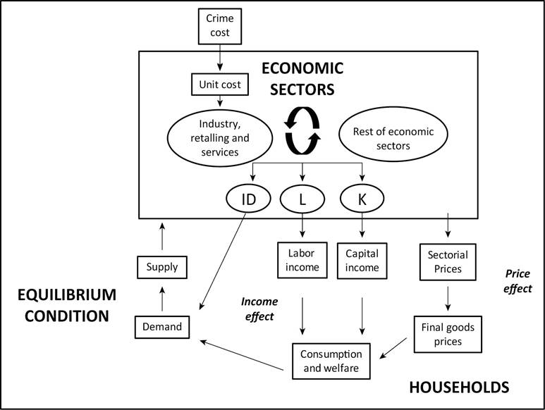
Source: Own elaboration.
Figure 2 Transmission of the Simulation 1: Forward pass-through of the crime tax
The negative price and income effects occasioned by the sales tax described in Simulation 1 are present in Simulation 2 but are smaller in magnitude. In addition, part of the cost of crime is introduced into the model as an increase in the cost of capital income relative to wages in the sectors. This produces a substitution effect, increasing the quantity demanded of labor (L) to the detriment of capital (K), resulting in a positive income effect on households, because labor income increases and a negative income effect on capital income. Therefore, there is a negative price effect, two negative income effects and a positive income effect. Even though the sign of the income effect is uncertain, we consider that in the aggregate, the negative effects will most likely dominate and reduce consumption demand, and thus, aggregate demand.
Due to the general equilibrium condition, aggregate supply decreases, causing a reduction in the demand for the intermediate inputs (ID), labor (L) and capital (K). This contracts the household disposable income and consumption, starting the latter process all at once, until it converges. This process is the same that is depicted in Figure 2 but adding a second transmission mechanism at the level of Labor and Capital incomes4.
In Simulation 3, the cost of crime faced by the commercial and service sectors is shifted forward, generating negative price and income effects on households. This leads to a reduction in consumption and economic activity. In addition, the industrial sector absorbs the cost of crime, generating a substitution effect in favor of labor and against capital, resulting in a positive income effect due to the increase in the labor income and a negative income effect due to the reduction in capital income. In the aggregate, we consider that the negative effects will dominate and that the consumption and economic activity will fall.
Results
Table 2 presents the effect of crime on basic macroeconomic indicators. Consumption change is between -7 and -8 % depending on the simulation, whereas value added and disposable income decline between 4 to 5 %. It is interesting to note that the contractions in the macroeconomic variables are greater to the extent that crime is partially absorbed in the sectors (i.e., Simulation 2) or exclusively in the industry (i.e., Simulation 3). The difference between Simulation 3, which has the largest effects, and Simulation 1, which represents the smallest estimates, is approximately 1%, except for the Capital Demand. When comparing Simulation 3 and Simulation 2, it is in the order of 0.3%.
Table 2 Aggregate effects of crime on the major macroeconomic variables of Mexico according to the different simulations
| Variable | Simulation 1 | Simulation 2 | Simulation 3 |
|---|---|---|---|
| Consumption | -6.70% | -7.00% | -8.30% |
| Disposable income | -4.10% | -4.40% | -5.20% |
| Saving | -4.20% | -4.80% | -5.60% |
| Investment | 0.00% | 0.00% | 0.00% |
| Capital Demand | -4.40% | -6.00% | -7.20% |
| Labor Demand | -4.20% | -2.90% | -3.40% |
| Gross Output | -3.60% | -3.80% | -4.50% |
| Value Added | -4.30% | -4.50% | -5.40% |
| Domestic output | -4.20% | -4.50% | -5.30% |
Source: Own elaboration.
In Simulations 2 and 3, in which the relative price of labor and capital is altered, a substitution effect is generated, increasing the quantity demanded for labor and reducing the quantity demanded for capital. Hence, we note that, in the aggregate, the demand for labor falls by less than the demand for capital. In contrast, in Simulation 1, where the relative price of primary inputs is not altered, the demand for labor and capital falls by similar percentages.
The sectors that are most affected across the three simulations are the commercial sector and the services sector, their domestic production falls between 4% to 6%. The industrial sector is in third place, with declines in production between 4% to 5%. When the cost of crime to businesses is shifted backwards, it primarily affects the industrial sector. The circular income flow mechanism causes the commerce and services sectors to be the most highly affected areas. The agricultural and governmental sectors are impacted indirectly, through the purchase-sale relationships of the intermediate inputs with the industrial, commercial and service sectors and by the reduction in household disposable income, which, in turn, implies a drop in the demand for consumer goods (see Table 3).
Table 3 Crime effects on the productive sectors of Mexico according to the different simulations
| Agriculture | Industry | Retailing | Services | Government | |
|---|---|---|---|---|---|
| Simulation 1 | |||||
| Capital demand | -3.30% | -3.70% | -5.20% | -4.90% | 0.00% |
| Labor demand | -3.30% | -3.70% | -5.20% | -4.90% | -0.10% |
| Value added | -3.30% | -3.70% | -5.20% | -4.90% | -0.10% |
| Domestic output | -3.30% | -3.70% | -5.20% | -4.90% | -0.10% |
| Consumer price index | 1.00% | 3.30% | 4.40% | 2.30% | 1.00% |
| Simulation 2 | |||||
| Capital demand | -3.70% | -6.10% | -6.50% | -5.90% | 0.00% |
| Labor demand | -3.70% | -0.50% | -3.80% | -4.20% | -0.10% |
| Value added | -3.70% | -4.30% | -5.00% | -5.00% | -0.10% |
| Domestic output | -3.70% | -4.30% | -5.00% | -5.00% | -0.10% |
| Consumer price index | 1.20% | 4.20% | 3.50% | 2.30% | 1.10% |
| Simulation 3 | |||||
| Capital demand | -4.40% | -8.50% | -6.10% | -5.90% | 0.00% |
| Labor demand | -4.40% | 2.40% | -6.10% | -5.90% | -0.10% |
| Value added | -4.40% | -5.20% | -6.10% | -5.90% | -0.10% |
| Domestic output | -4.40% | -5.20% | -6.10% | -5.90% | -0.10% |
| Consumer price index | 1.40% | 5.10% | 4.60% | 2.60% | 1.40% |
Source: Own elaboration.
The results in Table 4 reveal that when the costs of crime to businesses are fully shifted forward, the negative impact of crime on household consumption and income levels are more or less equal among all income quintiles. For example, the poorest households’ consumption drops 6.3%, while the richest ones’ consumption falls 6.8%, a marginal difference of half a percentual point. In this sense, when crime is modeled as a tax on production, it functions as a proportional tax.
Table 4 Major effects of crime on the income quintiles of Mexico according to the different simulations
| Variable I | I | II | III | IV | V |
|---|---|---|---|---|---|
| Simulation 1 | |||||
| Consumption | -6.30% | -6.40% | -6.50% | -6.60% | -6.80% |
| Disposable income | -3.80% | -3.80% | -3.90% | -4.00% | -4.30% |
| Cost of consumption bundle | 2.70% | 2.80% | 2.80% | 2.80% | 2.70% |
| Simulation 2 | |||||
| Consumption | -5.80% | -5.70% | -6.20% | -6.20% | -7.70% |
| Disposable income | -3.10% | -3.00% | -3.50% | -3.40% | -5.10% |
| Cost of consumption bundle | 2.90% | 2.90% | 2.90% | 2.90% | 2.80% |
| Simulation 3 | |||||
| Consumption | -6.90% | -6.80% | -7.40% | -7.30% | -9.10% |
| Disposable income | -3.70% | -3.50% | -4.10% | -4.10% | -6.00% |
| Cost of consumption bundle | 3.50% | 3.50% | 3.50% | 3.50% | 3.40% |
World Bank Enterprise Survey 2010. Note: I contain the 20% of the households with the lowest incomes and V the 20% of the households with the highest incomes Source: Own elaboration.
In contrast, in the second and third simulations, the negative impact on the consumption is larger in the higher income quintiles than in the poorest ones. In both simulations fifth quintile consumption drops 2 percentual points more than the first quintile because the richest families are the primary owners of capital income, which, in these simulations, is reduced. The results reveal that when a part of the crime burden falls on capital, the tax becomes slightly progressive.
The previous results are due to the negative income effect caused by the costs of crime. To the extent that costs are passed backwards, the income effect becomes stronger and affects, to a greater extent, households in the fifth income quintile. It should be noted that most of the capital income is concentrated in that quintile (64.2%).
Conclusions
We present a general equilibrium model for Mexico that includes the cost faced by firms as a result of crime. The exercise illustrates that there is a significant insecurity cost faced by firms in Mexico; it represents between 4% and 5% of the total value added.
In methodological terms, this study shows that the estimates are sensitive to the ability of firms to shift the tax forward to the consumer or backward to the capital factor. In general, we find that the largest contractions occur when the system is highly distorted. Similarly, when crime is modeled as a sales tax, the effect on relative household income approximates that of a proportional tax. The greater the share absorbed by a single sector (Simulation 3), the more it resembles a progressive tax.
However, it must be recognized that the modeling carried out in this investigation does not consider the dynamics of the process. For this reason, we cannot isolate the effect of crime on productive investment and the long-term effects on the system. Similarly, the salient differences between the estimates of the costs of crime from the World Bank Survey compared to the INEGI survey lead us to believe that the calibration of the tax rates that crime entails need to be further refined.
Another important limitation of our study is that it does not consider the cost of insecurity in the primary sector. This is because no survey that addresses insecurity in Mexico includes the agricultural sector. In this sense, our estimates should be considered as a lower limit. Clearly, there is an opportunity to estimate the cost of crime in this sector, one option may be to calibrate the cost of crime based on reports of robberies or homicides in rural areas, another is to take estimates from states where this sector is dominant. An additional way of sizing the shock in the agricultural sector caused by crime consists of estimating an econometric model where the variable to be explained is the consumer price index for agricultural products and considering a measure of crime as independent variable.
An additional future line of research consists in estimating the net economic effect of crime on enterprises. For this, the income of the families of the criminals and their consumption pattern according to economic sector are required, information that until now is not available in the case of Mexico.

