


 nueva página del texto (beta)
 Inglés (pdf)
 Artículo en XML
 Referencias del artículo
 Enviar artículo por email
 Citado por SciELO
  Similares en
SciELO
Similares en
SciELO 
 Permalink
1. Introduction
In Mexico, student enrollment in private universities experienced a sustained increase between 2005 and 2019. In that period, the number of students who enrolled in these universities more than doubled, from around 786 thousand to slightly more than 1.5 million students, i.e. an increase of 93.8%. As a result, the percentage of private university enrollments in the country’s total enrollment increased from 32.7% in 2005 to 35.7% in 2019 (Figure 1).
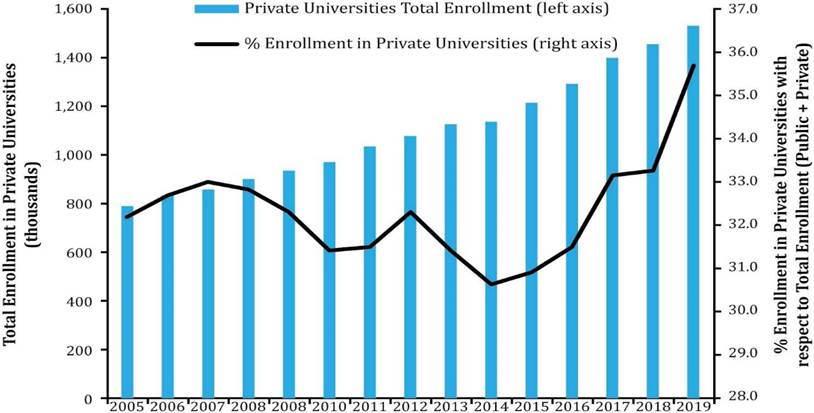
Figure 1 Total Enrollment in Private Universities and % Enrollment Private Universities with respect to Total Enrollment (Public+Private) 2005-2019
In this context, this paper will focus on studying the recent pattern of tuition inflation in private higher education. Several factors highlight the relevance of studying this phenomenon, as well as its potential determinants. The first factor is that the educational services of private universities are part of the bundle of goods and services used for the calculation of core inflation.1 Hence, examining the dynamics of their prices, as reflected in the Private Universities Tuition Index, contributes to the understanding of the overall inflation as measured by the National Consumer Price Index (CPI). This is especially relevant in the period 2015-2019, when its pattern experienced periods of acceleration and deceleration, both at the national and regional levels. In this regard, the available information shows that after reaching a rate of 4.2% between December 2015 and December 2016, during the same periods in 2017, 2018 and 2019 the education services annual inflation rate of private universities accelerated, reaching levels of 4.6, 5.2 and 4.7%, respectively (Figure 2). It is also observed, for the same periods, that the evolution of inflation in the Private Universities Tuition Index was heterogeneous across the country’s regions.2 For example, the acceleration observed between 2016 and 2018 was more significant in the centre-north and centre; in the south, an acceleration was also observed in that period, albeit of a lesser magnitude, while in the north, a temporarily higher inflation was observed in 2016. Between December 2018 and December 2019, the annual inflation rate decelerated in each region; however, in the north-central and central regions, average inflation for these educational services was higher than in 2016 (Figure 3). A second element underpinning the relevance of this work is that it will allow us to determine whether there are differences in the contribution of supply and demand factors to the recent evolution of these fees and to identify fac- tors behind these differences.
Source: Own elaboration with data from INEGI.
Figure 2 Price Index of Private Universities Variation December-December
Source: Own elaboration with data from INEGI.
Figure 3 Price Index of Private Universities by Region Variation December-December
Considering the above, the main objective of this paper is to identify the determinants of the dynamics of tuition inflation in private universi- ties in Mexico during the period of 2005-2019. The estimations are carried out within a framework of simultaneous equations given our specification of a model of inverse supply and demand functions. The estimation procedure considers two-stage (2SLS) and three-stage least squares (3SLS) with annual panel data at the state level for the period from 2005 to 2019. The paper contributes to the literature on the subject in Mexico since the results here discussed provide the first estimates of supply and demand elasticities for private higher education that take advantage of the panel data structure to capture phenomena attributable to the time series. Moreover, this structure allows us to identify the supply and demand factors that have contributed the most in explaining the dynamics of private tuition fees in the periods of interest, therefore contributing to a better understanding of the dynamics of the National Consumer Price Index (CPI) through core inflation.
The results suggest show that while the contribution of demand variables has been positive and relatively stable, the contribution of supply variables, although more fluctuating, has also been much higher than that associated to demand variables. The estimated model also shows that in the sub-period of the recent increase in private tuition fees (2016-2018), “skilled employment” stands out as the demand factor that contributed the most to the sustained increase in the acceleration, suggesting that a more intensive use of this type of employment encourages certain segments of the population to pursue higher education. On the supply side, the main contributing factors were the “average price of medium-voltage electricity” and the “price of communication services”. In turn, the drop in economic activity, given by the percentage change in the Quarterly Indicator of State Economic Activity (ITAEE by its acronym in Spanish), is the factor that contributed the most, both on the supply and demand side, to explain the slowdown in the price of private university tuition observed in the 2018-2019 sub-period.
The rest of the paper is structured as follows. Section 2 presents a brief review of the literature on the determinants of private university tuition prices; Section 3 describes the variables to be used to estimate the equilibrium prices of private universities in the period under study and presents the econometric model used to estimate them; Section 4 shows the estimation results; and Section 5 provides the final considerations.
2. Literature Review
The literature on the determinants of university tuition fees is mainly based on the US experience, and recognises a number of demand and supply factors that influence the behaviour of tuition fees. For example, Clotfelter (1990) reports that the higher profitability of university education compared to lower levels of education, as well as increases in wages and family wealth, boosts the demand for private higher education services and, with it, their fees. Later, the same author studies supply factors, finding that universities’ efforts to offer their students better services (library, health, sanitation, library, administrative, etc.), new equipment and facilities, as well as financial support for outstanding low-income students, tend to increase tuition fees (Clotfelter, 1996). Baumol (1967) mentions, at a theoretical level, that increases in teachers’ salaries also represent a potential risk factor for fee increases in educational services.
Paulsen (1991) is among the first to estimate, using a simultaneous equations framework, the effect of supply and demand factors on the equilibrium fees of public and private universities in the United States. Among his findings, the author reports that, on the supply side, greater efforts by universities to reduce operating costs (electricity, cleaning, water, etc.) and greater federal and state support for public universities reduce the rate of tuition growth. On the demand side, he finds that increased market competition between public and private universities has a negative impact on the increase in tuition fees for both types of universities. In a more recent paper, Bundick and Pollard (2019) also estimated a simultaneous equation model of supply and demand for educational services at public and private universities and reported that tuition fee increases are essentially driven by supply-side factors. Specifically, they mention that higher payroll expenditures, both for professors and non-academic staff, as well as reductions in public resources allocated to these institutions, are the main factors that explain the variation in tuition fees.
Other demand factors have been linked to the evolution of tuition fees. For example, it has been pointed out that private universities, when identifying times when students have more support for financing their education, whether private or public, their tuition fees tend to rise, which could be explained by the intention of these institutions to appropriate a fraction of those resources (Epple et al., 2013; Gordon and Hedlund, 2016; Lucca et al., 2017).3
Other work has paid specific attention to demand factors related to market competition, adding to Paulsen’s (1991) finding that increased market competition between public and private universities reduces tuition inflation. For example, Larsen (1997) suggests that changes in tuition prices at private higher education universities in the United States may have been due to illegal exchanges of information that some institutions made around tuition fees in order to avoid competing with each other. Hoxby (1997a) proposes that public and private universities located in markets that moved rapidly from regional monopolistic structures to more open and competitive structures responded to this growing exposure to competition by increasing their tuition fees. This was in response to their need to cover the higher costs required to offer higher quality educational services.4
In the case of Mexico, some studies analyse aspects related to the determinants of demand for private higher education. For instance, Acosta (2005) provides an overview of the evolution of the sector between 1980 and 2003, describing its origins and regulatory framework; the expansion of the number of institutions, academic staff and enrollment; the organisation and representation of the sector, and funding and admissions policies. Buendía (2009) acknowledges that the study of private higher education in the country is limited despite the continued expansion and increased commercialisation of the sector. Finally, Ramírez (2011) discusses various elements that have contributed to the growth and differentiation in demand for private higher education. Among the factors to be highlighted, he mentions the role of public policies, market forces that encourage or inhibit the emergence of differentiated educational services in order to meet a growing demand, and other characteristics that influence access to private higher education. However, no references were found for Mexico on the determinants of the supply of such educational services, nor on their equilibrium prices.5 For the estimation procedure, we did not find information regarding competition factors among private universities, nor variables related to the financing that private universities offer to their students.
Considering the above, this paper represents a first attempt to explain the behaviour of tuition fees at private universities in Mexico. Given that the available information allows us to identify some supply and demand factors of these educational services, we estimated a simultaneous supply and demand equations model to obtain the factors to changes in equilibrium prices of these services.6 These estimates are then used to measure the contributions the different supply and demand factors to changes in equilibrium prices at the national and regional levels.
3. Econometric Model
Understanding the dynamics of private university tuition fees requires recognizing, as previously mentioned, that it is a product of the dynamics resulting from the interaction of supply and demand factors. On the supply side, factors such as increases in teachers’ salaries, or increases in the prices of basic inputs for the provision of educational services, such as electricity or communication services, may lead, in an otherwise constant fashion, universities to pass on these changes in the form of higher tuition fees.7 In turn, increases in the demand for university education associated with increased labour market pressure for skilled employment, or increases in the college-age segment of the population, may put upward pressure on the demand for such education and thereby increase the otherwise constant tuition fees of private universities.
To estimate the effect of demand and supply factors on the equilibrium price of private university tuition, in this paper we will specify an inverse supply and demand system for private university tuition by means of equations (1) to (3):
where Pit denotes the price of private university tuition, as measured by the Private University Price Index from the CPI; the superscripts S and D refer to supply and demand, respectively; the subscript i refers to the state and the subscript t to time. Total private university enrollment for the academic years 2005-2006 to 2019-2020 approximates the quantities offered and demanded for the private university educational services, QSit and QDit, whose coefficients α and β are expected to be positive and negative, respectively. In turn, αi and βi are the fixed effects that allow to control for all those characteristics of the states that do not change over time; αt and βt, represent time fixed effects; and y ϵSit and y ϵDiit represent the error terms related to the supply and demand equations, respectively. XSit y XDit in turn represent vectors of variables that influence the supply of and demand for private higher education, respectively.8
On the supply side, we consider the fact that changes in the input costs can be transferred by private universities to the costs of their tuition fees. Thus, the vector XSit includes the costs associated with electricity consumption for use in the commercial and services sector, which were estimated with information from the Federal Electricity Commission (CFE). This source of information was used since there is no electricity producer price index available by state. Thus, the CFE information was used to calculate the variable (i) average price per kilowatt-hour of medium voltage high demand electricity (GDMTH).9 It also includes (ii) a communication services price index, associated with the cost of telecommunications services and composed of the following set of CPI generics: internet, telephony and pay TV packages; internet service, mobile telephone service and fixed telephone service. The data for this variable is obtained from the National Institute of Statistics and Geography (INEGI) and aims to capture a cost component of the provision of private university services. Also included is (iii) a variable associated with the possible cost of payroll expenditure.10 Specifically, it includes the annual variation of the base salary contribution of the sector “Academic teaching, training, scientific research and dissemination services” to the Mexican Social Security Institute (IMSS).
It is also necessary to consider variables which also control the likely effects that changes in the availability and quality of public university education services may have, directly or indirectly, on the price of tuition fees at private universities. To this end, we consider (iv) the enrollment rate of public universities, obtained from the National Association of Higher Education Universities (ANUIES); and (v) the federal budget allocated to public universities, obtained from the Database on Subsidies to Public Universities (Ordorika and Rodríguez, 2019) up to 2018, and for 2019 the information was obtained from the Transparency and Accountability Platform of the Ministry of Public Education (SEP). The first one aims to capture the effect that a greater presence of public universities would exert on the tuition prices of private universities, anticipating that a greater presence of public universities, reflected in their market share, that would tend to reduce the price of private universities. The second would capture the fact that a higher budget of public universities reflected, for instance, by improvements in the quality of public universities’ educational services, it would incentivise private universities to improve the quality of their services as well, thus raising their costs and, possibly, their prices. Finally, (vi) a Quarterly Indicator of State Economic Activity (ITAEE) as provided by INEGI, is included in order to control for general conditions of state economic activity that could influence pricing at the aggregate level.
On the demand side, the vector XD considers (i) the total employed population with a degree equal to or higher than a bachelor’s degree. Here, the employment of skilled labor reflects the possibility that a greater intensity in the use of skilled human capital may encourage certain segments of the population to study higher education, thus raising the demand for this level of education and, with it, tuition fees. It also includes (ii) the quotient of wages of bachelor’s degree graduates to wages of high school graduates, in order to control for the difference in wages of skilled and unskilled labour, anticipating that the larger the difference, the greater the incentives to demand more education. The data for these two variables is obtained from the National Occupation and Employment Survey (Encuesta Nacional de Ocupación y Empleo, ENOE). In addition, we added (iii) the annual variation of the IMSS contribution base salary of the sector “Academic teaching, training, scientific research and dissemination services”. These calculations are based on information from the Mexican Social Security Institute (IMSS). This variable, from the demand side, aims to capture the incentive for a higher demand of higher education in the light of increases in wage levels in the education sector, which is intensive in skilled labour. Also included is (iv) the number of high school graduates, which approximates the possible price effect of the demographic dynamics of the segment of the population that demands higher education in each academic cycle, information obtained from the SEP. In this case, too, higher demographic pressure is expected to have an upward effect on prices.
Also included, with data from ANUIES, two variables related to enrollment conditions in public universities: (v) the number of new applications to public universities, which is employed as an indicator of demand pressures for higher education, and (vi) the enrollment rate in higher education at public universities, used as an indicator of demand pressure for higher education. In this respect, it would be expected that higher levels of applications to public universities would tend to inhibit demand for higher education from private universities and thus put downward pressure on fees. However, the effect could be positive to the extent that this variable is also reflected in a higher demand for higher education. In addition, a higher effective enrollment rate of public universities may suggest that they are attracting a larger market share than private universities, negatively affecting the demand for higher education in private universities and thus could be associated with downward pressures on the cost of private tuition fees. Finally, (vii) the ITAEE is considered as a demand factor, seeking to capture the effect of state economic activity on the demand for private university higher education.
It is worth mentioning that in the estimation, all variables in the supply and demand vectors, Xit and Xit, are expressed in logarithms, with the exception of the change in the base contribution wage and the public university enrollment rate.11
Since the prices and quantities are determined simultaneously by the interaction of supply and demand functions, an ordinary least squares (OLS) estimation fails to identify them correctly, which could lead to biased estimators (Wooldridge,1996, 2010). A solution to this problem is to identify a set of factors (A) that affect supply conditions (costs) without affecting demand; or a set of factors (B) that affect demand without affecting supply conditions (costs). Factors of type (A) help to identify the demand curve, while factors of type (B) help to identify the supply curve.
The sets of factors (A) and (B) can be used as tools for the estimation of both equations by means of, for example, two-stage least squares (2SLS). Thus, a set of factors that reflect supply-side impacts (costs), but do not affect demand, will be used as instruments for estimating the demand function, while a set of factors that capture demand-side impacts, but do not affect supply conditions, is used for estimating the supply function (Rasmusen, 2007). In this way, it is possible to estimate each supply and demand equation separately, without making use of all the information contained in the detailed specification for the rest of the model. In this respect, Baum et al. (2002) argue that in order to correctly specify demand and supply functions using instrumental variables, the following two criteria need to be satisfied:
Relevance of the instrument: Intuitively, this requirement implies that since we want to use the instrument to represent our variable of interest, these variables must be strongly correlated. One way to assess the relevance of the instrument is through the F-statistic resulting from the estimation in the first stage, which should ideally be greater than 10.
Exogeneity or exclusion restrictions: This criterion implies that the instrument is not correlated with the error term and the only effect that the model will identify is the indirect effect of the variable of interest that is being instrumented. If the instruments are not exogenous, then 2SLS estimates are inconsistent. Furthermore, given the possibility of using more than instrument to correct specify the demand and supply curves, a test of overidentification restriction should also be considered. Empirically, test of overidentifying restrictions is important because it allows accounting for two issues simultaneously: a) whether the instruments are uncorrelated with the error term, and b) whether the equation is misspecified and that one or more of the excluded exogenous variables should in fact be included in the structural equation. Note that a significant test statistic could represent either an invalid instrument or an incorrectly specified structural equation. In practice, Hansen’s J statistic helps assess the validity of the instruments12.
Considering the above, we use the log of (a) applications to public universities, (b) the number of high school graduates, (c) the ratio of undergraduate wages to high school wages, and (d) the employment of skilled labour as instruments for the estimation of supply. The variables used as instruments for the estimation of demand are, in turn, the logarithms of (a) the average price per kilowatt-hour of medium voltage high demand electricity, (b) the price index of communications, and (c) the federal public budget allocated to public universities. As shown in the results section, the selection of these instruments fulfills the requirements above described: relevance of the instrument and exogeneity conditions.
Two estimation techniques are used to estimate the effects of demand and supply factors on the equilibrium cost of private university tuition. The first is two-stage least squares (2SLS), where endogenous explanatory variables are replaced by linear combinations of predetermined variables, or instruments. The second proposed estimation method is three-stage least squares (3SLS), which makes it possible to jointly estimate the system of equations in their structural form. It is therefore a complete information method that requires the specification of each of the equations of the system. This method starts from a correct specification of both equations in order to obtain the equilibrium price and quantity, estimating the supply and demand functions jointly, thus ensuring that QSit = QDit.13 It is worth mentioning that, by incorporating all the information of the system, the asymptotic efficiency of the estimates increases (ZellneryTheil, 1962; Alegre, 1993).
4. Results
Tables 1 and 2 show the estimation results for the supply and demand functions, respectively, using 2SLS and 3SLS. From the estimation with 2SLS, whose results are shown in the first columns of both tables, it is clear that the F-statistic of the first stage reaches values above 10, specifically 32.21 and 11.70, for the supply and demand equations, respectively, suggesting the relevance of the instruments proposed in both equations, as well as ruling out the presence of weak instru ments. Furthermore, the result of the Hansen’s J-statistic test suggests not rejecting the null hypothesis that instruments are not correlated with the error, thus pointing to the exogeneity of the instruments used in the identification in both the supply and demand equations.14
Table 1 Estimation of Suppy Equation1/ Two Stage Least Squares (2SLS) and Three Stage Least Squares (3SLS) Dependent Variable: Tution Price of Private Universities
| hola | 2SLS | 3SLS | |||
|---|---|---|---|---|---|
| Quantity | 0.026 (0.009) |
*** | 0.028 (0.009) |
*** | |
| Average Electricity Price (GDMTH) |
|
0.156 (0.075) |
*** | 0.093 (0.036) |
*** |
| Communications Price | 0.082 (0.038) |
** | 0.112 (0.032) |
*** | |
| ITAEE | 0.041 (0.022) |
* | 0.051 (0.023) |
*** | |
| Federal Budget to Public Universities | 0.003 (0.001) |
*** | 0.003 (0.001) |
*** | |
| Enrollment Rate of Public Universities | -0.001 (0.000) |
*** | -0.001 (0.000) |
*** | |
| Annual Variation of Base Salary | 0.046 (0.035) |
0.047 (0.040) |
|||
|
|
|
||||
| Observations | 480 | 480 | |||
| R-square | 0.188 | 0.957 | |||
| State Fixed Effects | YES | YES | |||
| Time Fixed Effects | YES | YES | |||
| F-statistic (1st stage) | 32.21 | ||||
| Hanen Overidentification Test (p-value) | 0.326 |
1/ Note: Heteroskedasticity robust standard errors in parentheses. Instruments: applications to public universities, the number of high school graduates, the ratio of undergraduate wages to high school wages, and the employment of skilled labour.
*, **, *** denote satatistical significance at 10%, 5% y 1%, respectively.
Source: Own elaboration with data from Ordorika and Rodríguez (2019), ANUIES, CFE, CONAPO, INEGI, IMSS, and SEP.
Table 2 Estimation of Demand Equation1/ Two Stage Least Squares (2SLS) and Three Stage Least Squares (3SLS) Dependent Variable: Tution Price of Private Universities
| 2SLS | 3SLS | |||
|---|---|---|---|---|
| Quantity | -0.115 (0.036) |
*** | -0.107 (0.033) |
*** |
| New Applications to Public Universities | 0.139 (0.030) |
*** | 0.133 (0.033) |
*** |
| High School Graduates | 0.080 (0.035) |
** | 0.042 (0.024) |
* |
| Ratio (Bachelor Wages)/(High School Wages) | 0.008 (0.017) |
0.009 (0.011) |
||
| Enrollment Rate of Public Universities | -0.001 (0.000) |
*** | -0.001 (0.000) |
** |
| Skilled Labor Force | 0.062 (0.036) |
* | 0.040 (0.024) |
* |
| ITAEE | 0.042 (0.032) |
0.053 (0.024) |
* | |
| Annual Variation of Base Salary | 0.058 (0.041) |
0.047 (0.040) |
||
|
|
||||
| Observations | 480 | 480 | ||
| R-square | 0.225 | 0.957 | ||
| State Fixed Effects | YES | YES | ||
| Time Fixed Effects | YES | YES | ||
| F-statistic (1st stage) | 11.70 | |||
| Hanen Overidentification Test (p-value) | 0.114 |
1/ Note: Heteroskedasticity robust standard errors in parentheses. Instruments: the average price per kilowatt-hour of medium voltage high demand electricity, the price index of communications, and (c) the federal public budget allocated to public universities.
*, **, *** denote statistical significance at 10%, 5% y 1%, respectively.
Source: Own elaboration with data from Ordorika and Rodríguez (2019), ANUIES, CFE, CONAPO, INEGI, IMSS, and SEP.
4.1 Supply Determinants
Taking the 3SLS estimation as a reference, the estimated coefficients of the supply equation in the second column of Table 1 indicate, as expected, that the one corresponding to “total enrollment of private universities” is positive and statistically significant.15
The estimates include heteroscedasticity-robust standard errors when estimation procedure correspond to 2SLS or 3SLS, while cluster-robust errors at the state level are estimated. For the calculation of the latter, the wild-bootstrap-t method is used due to the few clusters scenario that arises when considering the 32 states. For more details on the wild-bootstrap-t method, see Cameron et al. (2008). These results can be found in Tables 2A and 3A in the Appendix, which suggest robustness in the significance of the estimated variables indicated.
Also, as expected, the estimated coefficient estimates for “communications price” and “average price per kilowatt-hour of medium-voltage high demand electricity (GDMTH)” are positive and statistically significant. Only the estimated coefficient estimates for the annual change in the IMSS contribution base wage related to the employment of skilled labour were not statistically different from zero.
With respect to the variables that indicate that public universities compete with private universities, the coefficient of the “enrollment rate of public universities” is negative and statistically significant, indicating that if public universities have a larger market share, the tuition fees of private universities could be adjusted downwards.16 On the other hand, the coefficient of the public university budget variable exhibits a positive and statistically significant sign, indicating that in the face of possible improvements in the quality of public universities, private universities would have incentives to improve the quality of their services as well, thereby affecting costs and, possibly, raising fees. Likewise, the positive and statistically significant sign of the coefficient of the ITAEE would indicate that improvements in the general conditions of state economic activity could influence increases in the provision of private higher education, thus exerting an influence on the tuition fees of private universities.
4.2 Demand Determinants
In turn, the estimated demand equation shows, as expected, that the number of enrollments in private universities has a negative and statistically significant relationship with the tuition fees of private universities. Positive and statistically significant coefficients are also obtained for the remaining variables, with the exception of the variation in the base contribution wage, and the ratio of under-graduate to high school wages, whose coefficients were found to be statistically not significant. For example, these results suggest that a more intensive use of skilled employment would be associated with greater incentives for certain segments of the population to opt for higher education, leading to a higher demand for this service and thus pushing up tuition fees. In turn, the positive and statistically significant sign of the coefficient of new applications to public universities indicates that this variable is capturing a higher demand for university studies in general. The demographic factor, captured by the number of high school graduates in each academic year, suggests that increases in this segment of the population are reflected in increases in demand for private higher education, putting upward pressure on tuition fees.
Finally, the positive and statistically significant sign of the coefficient of the ITAEE variable suggests that a higher dynamic in the economic activity of the state would be associated with a higher demand for skilled and unskilled employment, the former being the one that could be associated with a higher demand for higher education and thus influencing tuition fees at private universities to rise.17,18
4.3 Estimated Contributions of Supply and Demand Factors to the Equilibrium Tuition Fees in Private Universities
The estimated supply and demand equations shown in Tables 1 and 2 make it possible to obtain the annual contributions, in percentage points (pp) and during the study period, of the different supply and demand variables on the cost of tuition fees at the national level. For this purpose, we considered the estimated coefficients in 3SLS of the variables that were statistically significant, the elasticity of each variable on the equilibrium price and the percentage variation of the different determinants of supply and demand during the period indicated.19,20 Thus, comparing the annual contributions of the demand and supply variables for the period 2005-2019, it is observed that both sets have exerted a persistent upward pressure on tuition fees. The effect of the demand variables has been more stable than that of the supply variables; however, it is the supply variables that have contributed the most to the increase in tuition fees (Figure 4).
Source: Own estimations with data from ANUIES, CFE, CONAPO, INEGI, IMSS, Ordorika and Rodríguez (2019) and SEP.
Figure 4 Annual Contribution to the Annual Variation of Equilibrium Prices in Private Universities Demand and Supply Factors, 2006-2019
Given the estimated parameters of the model, it is also possible to obtain the contribution of the different supply and demand factors during the period of greatest acceleration in university tuition fees, i.e. 2016-2018. This can be seen in Table 3, where the total supply and demand effects are obtained by multiplying columns (2) and (3) and adding the respective contributions of the fixed time effects. The results of these calculations yield a total estimated effect derived from the set of supply and demand variables of 4.80 pp, of which 3.77 pp correspond to the former and 1.03 pp to the latter; while the observed value of cumulative inflation by state between 2016 and 2018 of the cost of private university tuition was 4.19 pp.
Table 3. Estimation of the National Contribution of Demand and Supply Effects to the Annualized Tuition Price of Private Universities between December 2016 y December 20181/
| Coefficient | Elasticity | Annualized Rate1 | Effect on Inflación | ||
|---|---|---|---|---|---|
| Supply Variables | (1) | (∂P/∂D) (2) |
(%) (3) |
p.p. [(2)*(3)] |
|
| Average Electricity Price (GDMTH) | 0.093 (0.036) |
*** | 0.073 | 22.0 | 1.61 |
| Communications Price | 0.112 (0.032) |
*** | 0.089 | 0.9 | 0.08 |
| Enrollment Rate of Public Universities | -0.001 (0.000) |
*** | -0.001 | 1.5 | 0.00 |
| Federal Budget to Public Universities | 0.003 (0.001) |
*** | 0.003 | 2.8 | 0.01 |
| ITAEE | 0.051 (0.024) |
* | 0.051 | 0.8 | 0.04 |
| Demand Variables | |||||
| Skilled Labor Force | 0.040 (0.024) |
* | 0.046 | 5.2 | 0.24 |
| ITAEE | 0.053 (0.028) |
* | 0.042 | 0.8 | 0.03 |
| High School Graduates | 0.042 (0.024) |
* | 0.007 | 4.8 | 0.03 |
| New Applications to Public Universities | 0.133 (0.033) |
*** | 0.021 | 1.0 | 0.02 |
| Total Effect Supply Variables | 1.74 | ||||
| Supply Fixed Effects2/ | 2.04 | ||||
| Total Effect Supply | 3.77 | ||||
| Total Effect Demand Variables | 0.33 | ||||
| Demand Fixed Effects3/ | 0.71 | ||||
| Total Effect Demand | 1.03 | ||||
| Estimated Average Annual Total Effect | 4.80 | ||||
| Confidence Interval | (2.65-6.98) | ||||
| Observed Average Annual Inflation 1/ | 4.19 | ||||
1/ Note: The annualized rate is calculated as [(1+growth rate 2016-2018)^(1/2)]-1. 2/ Correspond to the supply anual average fixed effect.
3/ Correspond to the demand anual average fixed effect. Heteroskedasticity robust standard errors in parentheses.
*, **, *** denote statistical significance at 10%, 5% y 1%, respectively.
Among the factors that contributed the most to explain the change in the cost of private university tuition fees, on the supply side, the average price per kilowatt-hour of electricity for the medium-voltage high-demand tariff stands out, due to its percentage change during the 2016-2018 period, followed by the communications price index, given that its estimated elasticity is the largest. On the demand side, the skilled labour variable, which seeks to capture the intensity in the use of skilled human capital in the state labour market, is the factor that stands out, a result attributable, on one hand, to a positive estimated elasticity of the highest magnitude, and on the other, to a high percentage change.
The estimated model is also used to calculate the contributions of demand and supply factores over the inflation of private universities tuition but now at the regional level. This is based on the assumption that the estimated elasticities are common to all regions, but that each region may have faced differentiated changes in the supply and demand variables. Thus, the percentage changes of the supply and demand variables in the respective region for the given period are calculated. The convenience of the assumption that the elasticities are the same for all regions makes it possible to differentiate the estimated effect on tuition fee inflation derived only from regional impacts on those determinants, whether related to supply or demand, that turn out to be statistically significant.
Figure 5 shows these contributions between December 2016 and December 2018.21 The graph shows that the estimated total effect on tuition inflation in percentage points is largest in the central region (3.81+1.21=5.02), followed by the central north (3.89+1.07=4.96), north (3.58+1.12=4.70), and south (3.59+0.85=4.44) regions, in that order, consistent with the observed data.22 It can also be seen that the “average price of medium voltage high demand electricity” had a significant effect in all regions, although to a lesser extent in the north. It also stands out that in all regions the “employment of skilled labour” has the dominant effect among the demand factors, which is more noticeable in the centre, a region in which both the ITAEE and the “new applications to public universities” also contribute, pointing to a growing demand for higher education in this region.
Source: Own elaboration with information from ANUIES, CFE, CONAPO, INEGI, IMSS, Ordorika y Rodríguez (2019) and SEP.
Figure 5 Contribution of Demand and Supply Factors to the Evolution of Tuition Price between December 2016 and December 2018
Also noteworthy is the observed deceleration in tuition fees at the national level in the 2018- 2019 sub-period. To analyse the factors that contributed to this deceleration, a similar exercise was performed as in Table 5A in the Appendix. The results of the recalculations are presented in Table 4 23
Table 4 Estimation of the National Contribution of Demand and Supply Effects to the Annualized Tuition Price of Private Universities between December 2018 y December 2019
| Coefficient | Elasticity | Annual variation | Effect on Inflación | ||
|---|---|---|---|---|---|
| Supply Variables | (1) | (∂P/∂D) (2) |
(%) (3) |
p.p. [(2)*(3)] |
|
| Average Electricity Price (GDMTH) | 0.093 (0.036) |
*** | 0.073 | 7.69 | 0.56 |
| Communications Price | 0.112 (0.032) |
*** | 0.089 | -0.3 | -0.02 |
| Enrollment Rate of Public Universities | -0.001 (0.000) |
*** | -0.001 | 4.8 | 0.00 |
| Federal Budget to Public Universities | 0.003 (0.001) |
*** | 0.003 | 6.8 | 0.02 |
| ITAEE | 0.051 (0.024) |
* | 0.051 | -0.2 | -0.01 |
| Demand Variables | |||||
| Skilled Labor Force | 0.040 (0.024) |
* | 0.046 | 3.8 | 0.17 |
| ITAEE | 0.053 (0.028) |
* | 0.042 | -0.2 | -0.01 |
| High School Graduates | 0.042 (0.024) |
* | 0.007 | -2.40 | -0.02 |
| New Applications to Public Universities | 0.133 (0.033) |
*** | 0.021 | 11.8 | 0.25 |
| Total Effect Supply Variables | 0.54 | ||||
| Supply Fixed Effects2/ | 2.65 | ||||
| Total Effect Supply | 3.19 | ||||
| Total Effect Demand Variables | 0.40 | ||||
| Demand Fixed Effects3/ | 0.85 | ||||
| Total Effect Demand | 1.24 | ||||
| Estimated Average Annual Total Effect | 4.44 | ||||
| Confidence Interval | (2.49-6.35) | ||||
| Observed Average Annual Inflation 1/ | 4.73 | ||||
1/ Note: Heteroskedasticity robust standard errors in parentheses. 2/ Correspond to the supply anual average fixed effect.
3/ Correspond to the demand anual average fixed effect.
*, **, *** denote statistical significance at 10%, 5% y 1%, respectively.
Source: Own elaboration with data from Ordorika and Rodríguez (2019), ANUIES, CFE, CONAPO, INEGI, IMSS, and SEP.
As observed, on the demand side, the decline in the “number of high school graduates” contributed moderately to the slowdown in private tuition fees observed between 2018 and 2019, and that the decline in economic activity, due to the negative percentage change in the ITAEE, contributed to both the supply and demand aspects of the observed slowdown in the inflation of private university tuition fees. This result could suggest that, in a period of weak economic activity, applications to private universities would decrease, while on the supply side, it would be more difficult for private universities to transfer an increase in their costs to their tuition fees. On the other hand, among the supply factors that contributed the most to tuition inflation during the 2018- 2019 sub-period are the decrease in the percentage change in the “communications price index”, coupled with a lower increase in the “average price per kilowatt-hour of medium voltage high demand electricity.”
5. Final Considerations
This paper is a contribution to the study of the determinants of private university tuition fees in Mexico. Based on these estimates, it was possible to identify that the dynamics of equilibrium prices of private university tuition fees in Mexico during the period 2005-2019 responded to both supply and demand factors. It can also be observed that demand factors had a relatively stable contribution to private university tuition fee inflation over the estimated period, although this is much lower than that attributable to supply factors.
The estimates also suggest that for the 2016- 2018 sub-period, the supply factors that contributed the most to the increase in tuition fees were the “price of medium voltage electricity” and the “price of communication services.” On the demand side, the contribution of “skilled employment” stood out, suggesting that a more intensive use of this factor stimulated demand for higher education and exerted upward pressure on tuition fees. The estimates also indicate for this period that the sum of the estimated supply and demand effects on tuition fees was highest in the central region, followed by the north-central, northern and southern regions. In all of them, it can be seen that “medium voltage electricity prices” had an important effect, although to a lesser extent in the north. Also noteworthy is that in all the regions “employment of skilled labour” has a dominant effect among the demand factors, but this is most noticeable in the centre, where the ITAEE and “applications to public universities” also contribute, suggesting a growing demand for higher education in this region. In turn, the decline in the “number of high school graduates” contributed, albeit modestly and on the demand side, to explain the slowdown in the cost of tuition fees at private universities in the 2018-2019 sub-period.
Finally, it is important to note that this study uses information aggregated by state, given that this is the information available at the time. This fact represents a limitation as it precludes to analyze the role associated with the characteristics of each private sector higher education institution, such as the quality of their professors, the quality of their facilities, their size, location, the characteristics of the financial support they offer to their students, timetables, local effects of competition, among others, and which may be relevant to explain the evolution of tuition fees at private universities.
This paper also recognizes that prices in the private university market might be discriminatory; from which each student may pay a different price. This is because tuition prices might be attached to financing, scholarships, and progress by credit burden decisions. Also, it might be the case that some private are non-profit organizations which means that all profits are not turned into dividends. In this sense, lacking working with individual level data or administrative records limits the analysis for undertaking, for example, a counterfactual analysis to assess the implications either of a tax or a subsidy in this market; determine the implications of an increasing automatization or determine the consequences of cleaner and cheaper technologies. The empirical analysis shall test for estimation implications (consistency and biasness) of the factors above referred.
To the extent that this information is generated and incorporated in future econometric studies, a better understanding of this relevant component of core inflation dynamics in Mexico will be possible.

