


 nova página do texto(beta)
 Inglês (pdf)
 Artigo em XML
 Referências do artigo
 Enviar este artigo por email
 Citado por SciELO
  Similares em
SciELO
Similares em
SciELO 
 Permalink
Introduction
Over the past decades, the Mexican population has undergone the epidemiological transition, from a primarily preventable causes of death due to infection and other preventable diseases, to the emergence of an increasing degenerative causes of death. Along these lines, one primary concern is the rise in obesity and type II Diabetes (Diabetes from now on). Associated with these increasing morbidity rates, Mexico has experienced a significant expansion of the Diabetes mortality rates (Barquera, Campos-Nonato, & Hernández-Barrera, 2013).
Diabetes prevalence has increased among adults of every age group and it has been one of the most important causes of death in Mexico since 2000, being at least 1.6 times as often the underlying cause of death (Bustamante-Montes, Lezama-Fernández, Fernández-De Hoyos, Villa-Romero, & Borja-Aburto, 1990). These changes have had significant negative effects on life expectancy in Mexico (Agudelo-Botero & Dávila-Cervantes, 2015; Dávila-Cervantes & Pardo, 2014; Palloni, Beltrán-Sánchez, Novak, Pinto, & Wong, 2015).
The Diabetes prevalence pattern in Mexico has been extremely heterogeneous; unlike the United States, it has shown that the epidemiological transition across states has not occurred simultaneously. A group of Mexican researchers called this phenomenon the “polarization of the transition” (Frenk, Bobadilla, Sepúlveda, & López, 1989) where different regions of the country are experiencing the epidemiological transition in different ways (Frenk & Chacón, 1991a, 1991b).
There is evidence of the recent trends in the prevalence of Diabetes and its risk factors in national health surveys (Villalpando, Shamah-Levy, Rojas, & Aguilar-Salinas, 2010). From 1993 to 2006, the prevalence of Diabetes increased from 6.7% to 14.4%; to note, the relative change in mortality for the period 1980-2000 shows that the most significant increase has been mainly in the southern central and Mexico City regions (Barquera, Tovar-Guzmán, Campos-Nonato, González-Villalpando, & Rivera-Dommarco, 2003). This dynamic predicts larger increments in the near future for Diabetes morbidity and mortality.
At national level, the adults aged 20 years and above, with overweight and obesity was 75.2% (39.1% overweight and 36.1% obesity) in 2018, compared to 71.3% in 2012. Likewise, the states that presented the higher percentages were Campeche, Tamaulipas, Hidalgo, Mexico City and Nuevo Leon. The percentage of the population aged 20 years and above with a diagnosis of Diabetes in 2012 was 9.2% (6.4 million); by sex, 9.7% were women and 8.6% men; in 2018, it was 10.3% (8.6 million), 11.4% females and 9.1% males (Instituto Nacional de Estadística y Geografía [INEGI], Instituto Nacional de Salud Pública [INSP], & Secretaría de Salud [SS], 2019).
The purpose of the current study is to propose an objective approach to allocate resources, based on hierarchical forecasts of Diabetes mortality to 2030, using the Hyndman and Athanasopoulos (2018) method. The hierarchical time series model allows to forecast the number of deaths by Diabetes based on sub-domains of the population. It is important to recognize that the hierarchical structure is absolutely flexible and it depends on the analyst’s criteria and the goal pursued.
This paper is organized as follows. The next section is devoted to the economic burden of Diabetes and different estimates made for the mexican case. In the next section, the methodology is presented, describing how data is handled and how the model is established, in accordance with the proposed hierarchical structure. Then, the results of the forecasts are exposed from the first to the last level of the mentioned structure. Here, it is evident the coherence among the forecasts. Afterwards, the main conclusions are described and justified to highlight a new public health policy.
Estimates economic burden of Diabetes
Diabetes has become one of the leading public health challenges of the twenty-first century due to the large economic burden and its adverse impact on the overall health of the population. This emerging morbid condition has placed increasing costs on the Mexican healthcare system. Its economic burden affects a wide range of variables, including economic and human development, as well as the conditions of equity and poverty (Barquera et al., 2013). In other words, its economic impact encompasses the direct costs associated with spending on health care, that is medical services and drugs, and indirect costs of the disease that relate to the effect of premature mortality and disability of a person to participate effectively in the labor market.
The 2013 estimates suggest that the economic burden of Diabetes was about 2.25% of the mexican GDP. This amount is greater than the actual annual growth of the Mexican economy of 2.1%, registered by INEGI at the end of 2014, and the one projected for 2021. The direct costs of Diabetes were estimated at $179,495.3 million pesos in 2013 (Barraza-Lloréns et al., 2015). Likewise, financially speaking, comparing the economic impact in 2012 versus 2010 Arredondo and Reyes (2013) estimated a 33% increase in costs associated to this public affection. Thus, they posited the need to review the current organization of the mexican health system, to move from a curative health care mode to preventive models that enable a better way to deal with the expected challenges.
Most recently, Arredondo, Orozco, Alcalde-Rabanal, Navarro, and Azar (2018) estimate the economic burden of the health services demand due to Diabetes and hypertension for the mexican insured and uninsured population in five regions. According to their results, between 2013 and 2018, the economic burden of both diseases increased between 58%-66%. They also argue that, based on their forecasts, on each of the analyzed regions, to address these diseases, the authorities will require between 13% and 15% of the public health budget for the uninsured population and between 15% and 17% for the insured population.
To determine trends related to the economic burden from Diabetes, Arredondo et al. (2019) developed a longitudinal analysis. This analysis generated two key findings: there was a 26% increase in the economic burden from incidence from 2016 to 2018, and the total amount allocated to treat Diabetes in 2017 was $9 684 780 574 (us dollars). Thus, they suggest reviewing and rethinking strategies of prevention, planning, organization and resource allocation.
The same analysis of economic burden of Diabetes in the elderly was made by Arredondo (2020). He compared the economic burden for 2020 versus 2022 and concluded that the increase was estimated at 29%. He also pointed that amid the coronavirus 2019 pandemic, there is a serious complication to achieve the scope of universal coverage for diabetics in Mexico. It is worth mentioning that based on the aforementioned literature, there is no proposal for the objective allocation of resources to face the economic burden, based on the deaths that occur by sub-domains of the population, and which is considered a relevant contribution of this paper.
Methodology
Data
Data was extracted from two sources. First, the mortality data are taken from the INEGI and the SS (1985-2017); individual level micro-data available at https://cutt.ly/8wMbkfu. Second, official population estimates are obtained from the Mexican population council (Consejo Nacional de Población [CONAPO], 2019) available at https://cutt.ly/JwMn6p0. From the INEGI data, data counts of deaths by Diabetes-related causes (ICD-10 codes) were obtained for years 1985 to 2017 (the most recent data available). The (mid-year) anual population estimates data from CONAPO for the 1985 to 2030 period were considered. All these data were classified by marginalization and sex. The datasets analyzed and generated during the current study are available in Table 1.
Table 1 Deaths by Diabetes and Population
| Deaths (thousands) | Population (millions) | |||||||||||||||||||||||||||||||
|---|---|---|---|---|---|---|---|---|---|---|---|---|---|---|---|---|---|---|---|---|---|---|---|---|---|---|---|---|---|---|---|---|
| Year | Total | HI | LO | ME | VH | VL | HIM | HIW | LOM | LOW | MEM | MEW | VHM | VHW | VLM | VLW | Total | HI | LO | ME | VH | VL | HIM | HIW | LOM | LOW | MEM | MEW | VHM | VHW | VLM | VLW |
| 1985 | 20.41 | 4.26 | 5.66 | 2.77 | 1.04 | 6.68 | 1.87 | 2.39 | 2.43 | 3.23 | 1.23 | 1.54 | 0.44 | 0.60 | 3.00 | 3.68 | 76.03 | 18.55 | 22.22 | 12.44 | 7.98 | 14.84 | 9.22 | 9.33 | 11.04 | 11.18 | 6.20 | 6.23 | 3.99 | 3.99 | 7.27 | 7.57 |
| 1986 | 23.03 | 5.05 | 6.58 | 3.10 | 1.10 | 7.20 | 2.18 | 2.87 | 2.86 | 3.72 | 1.35 | 1.74 | 0.45 | 0.65 | 3.03 | 4.17 | 77.69 | 18.94 | 22.80 | 12.77 | 8.24 | 14.95 | 9.40 | 9.54 | 11.32 | 11.48 | 6.36 | 6.41 | 4.11 | 4.13 | 7.33 | 7.62 |
| 1987 | 23.97 | 5.44 | 6.50 | 3.21 | 1.12 | 7.71 | 2.33 | 3.11 | 2.76 | 3.74 | 1.38 | 1.83 | 0.49 | 0.63 | 3.29 | 4.42 | 79.34 | 19.32 | 23.37 | 13.10 | 8.50 | 15.04 | 9.58 | 9.74 | 11.60 | 11.77 | 6.52 | 6.58 | 4.24 | 4.26 | 7.38 | 7.67 |
| 1988 | 24.98 | 5.43 | 7.26 | 3.55 | 1.23 | 7.50 | 2.40 | 3.04 | 3.19 | 4.07 | 1.56 | 1.99 | 0.53 | 0.70 | 3.20 | 4.30 | 80.97 | 19.70 | 23.94 | 13.44 | 8.76 | 15.13 | 9.76 | 9.94 | 11.88 | 12.07 | 6.68 | 6.76 | 4.36 | 4.40 | 7.42 | 7.70 |
| 1989 | 25.57 | 5.46 | 7.45 | 3.68 | 1.29 | 7.68 | 2.41 | 3.05 | 3.23 | 4.22 | 1.61 | 2.07 | 0.55 | 0.74 | 3.39 | 4.29 | 82.58 | 20.07 | 24.52 | 13.77 | 9.02 | 15.20 | 9.93 | 10.14 | 12.16 | 12.36 | 6.83 | 6.93 | 4.48 | 4.53 | 7.46 | 7.74 |
| 1990 | 25.71 | 5.34 | 7.71 | 3.61 | 1.25 | 7.79 | 2.29 | 3.05 | 3.34 | 4.37 | 1.64 | 1.97 | 0.53 | 0.72 | 3.38 | 4.42 | 84.17 | 20.43 | 25.11 | 14.07 | 9.22 | 15.35 | 10.10 | 10.33 | 12.45 | 12.66 | 6.98 | 7.09 | 4.58 | 4.64 | 7.54 | 7.81 |
| 1991 | 27.07 | 5.76 | 8.15 | 4.00 | 1.35 | 7.80 | 2.54 | 3.23 | 3.59 | 4.56 | 1.80 | 2.20 | 0.57 | 0.78 | 3.46 | 4.34 | 85.75 | 20.75 | 25.73 | 14.34 | 9.35 | 15.57 | 10.25 | 10.50 | 12.75 | 12.98 | 7.11 | 7.23 | 4.64 | 4.71 | 7.65 | 7.93 |
| 1992 | 28.26 | 5.98 | 8.48 | 4.24 | 1.44 | 8.11 | 2.63 | 3.35 | 3.78 | 4.71 | 1.90 | 2.35 | 0.63 | 0.81 | 3.62 | 4.49 | 87.31 | 21.08 | 26.35 | 14.61 | 9.48 | 15.79 | 10.40 | 10.67 | 13.05 | 13.30 | 7.24 | 7.37 | 4.70 | 4.78 | 7.75 | 8.04 |
| 1993 | 29.52 | 6.30 | 8.85 | 4.59 | 1.62 | 8.15 | 2.69 | 3.61 | 3.91 | 4.94 | 1.99 | 2.60 | 0.68 | 0.94 | 3.58 | 4.58 | 88.85 | 21.39 | 26.97 | 14.87 | 9.61 | 16.01 | 10.55 | 10.84 | 13.35 | 13.62 | 7.36 | 7.51 | 4.76 | 4.85 | 7.86 | 8.15 |
| 1994 | 30.26 | 6.64 | 8.98 | 4.45 | 1.84 | 8.36 | 2.84 | 3.79 | 4.00 | 4.98 | 1.94 | 2.51 | 0.79 | 1.06 | 3.69 | 4.67 | 90.36 | 21.70 | 27.59 | 15.13 | 9.73 | 16.22 | 10.69 | 11.00 | 13.65 | 13.94 | 7.49 | 7.64 | 4.82 | 4.91 | 7.96 | 8.26 |
| 1995 | 33.25 | 7.17 | 10.11 | 5.11 | 1.99 | 8.88 | 3.15 | 4.02 | 4.48 | 5.63 | 2.27 | 2.84 | 0.86 | 1.13 | 3.89 | 4.99 | 91.84 | 21.99 | 28.20 | 15.38 | 9.85 | 16.42 | 10.83 | 11.16 | 13.95 | 14.25 | 7.61 | 7.77 | 4.87 | 4.98 | 8.05 | 8.36 |
| 1996 | 34.80 | 7.79 | 10.52 | 5.32 | 2.12 | 9.05 | 3.45 | 4.34 | 4.74 | 5.77 | 2.38 | 2.94 | 0.91 | 1.21 | 3.95 | 5.10 | 93.29 | 22.27 | 28.81 | 15.62 | 9.99 | 16.61 | 10.95 | 11.31 | 14.25 | 14.57 | 7.72 | 7.90 | 4.94 | 5.05 | 8.15 | 8.46 |
| 1997 | 35.97 | 7.71 | 11.25 | 5.54 | 2.31 | 9.16 | 3.30 | 4.41 | 5.07 | 6.18 | 2.41 | 3.13 | 0.98 | 1.33 | 4.10 | 5.07 | 94.72 | 22.52 | 29.42 | 15.84 | 10.15 | 16.80 | 11.06 | 11.46 | 14.54 | 14.87 | 7.82 | 8.02 | 5.01 | 5.14 | 8.25 | 8.55 |
| 1998 | 41.78 | 8.81 | 12.86 | 6.69 | 2.63 | 10.79 | 3.84 | 4.97 | 5.73 | 7.13 | 3.02 | 3.67 | 1.08 | 1.55 | 4.91 | 5.88 | 96.12 | 22.76 | 30.02 | 16.05 | 10.31 | 16.98 | 11.15 | 11.61 | 14.83 | 15.18 | 7.91 | 8.13 | 5.08 | 5.23 | 8.34 | 8.64 |
| 1999 | 45.59 | 9.92 | 14.13 | 7.11 | 2.93 | 11.50 | 4.25 | 5.67 | 6.34 | 7.79 | 3.15 | 3.96 | 1.26 | 1.67 | 5.24 | 6.26 | 97.48 | 23.00 | 30.61 | 16.25 | 10.47 | 17.15 | 11.24 | 11.76 | 15.12 | 15.49 | 8.00 | 8.25 | 5.15 | 5.32 | 8.43 | 8.72 |
| 2000 | 46.55 | 10.55 | 13.97 | 7.27 | 3.08 | 11.69 | 4.54 | 6.01 | 6.43 | 7.54 | 3.25 | 4.02 | 1.31 | 1.77 | 5.31 | 6.38 | 98.79 | 23.23 | 31.15 | 16.45 | 10.60 | 17.35 | 11.33 | 11.89 | 15.38 | 15.77 | 8.09 | 8.36 | 5.20 | 5.40 | 8.53 | 8.82 |
| 2001 | 49.87 | 11.71 | 15.00 | 7.72 | 3.40 | 12.04 | 5.11 | 6.60 | 6.80 | 8.20 | 3.47 | 4.26 | 1.47 | 1.93 | 5.47 | 6.56 | 100.11 | 23.46 | 31.66 | 16.66 | 10.72 | 17.60 | 11.43 | 12.03 | 15.62 | 16.04 | 8.19 | 8.47 | 5.25 | 5.47 | 8.65 | 8.95 |
| 2002 | 54.85 | 12.66 | 16.50 | 8.69 | 3.94 | 13.06 | 5.71 | 6.95 | 7.72 | 8.78 | 3.90 | 4.79 | 1.75 | 2.19 | 6.07 | 6.98 | 101.49 | 23.71 | 32.20 | 16.88 | 10.84 | 17.86 | 11.54 | 12.17 | 15.88 | 16.32 | 8.29 | 8.59 | 5.30 | 5.54 | 8.78 | 9.08 |
| 2003 | 59.14 | 13.66 | 17.84 | 9.24 | 4.18 | 14.22 | 6.01 | 7.65 | 8.24 | 9.60 | 4.15 | 5.10 | 1.84 | 2.35 | 6.53 | 7.68 | 102.89 | 23.97 | 32.74 | 17.10 | 10.97 | 18.12 | 11.65 | 12.32 | 16.14 | 16.60 | 8.39 | 8.71 | 5.36 | 5.61 | 8.91 | 9.21 |
| 2004 | 62.23 | 14.51 | 18.54 | 9.92 | 4.39 | 14.88 | 6.42 | 8.10 | 8.60 | 9.93 | 4.50 | 5.42 | 1.89 | 2.51 | 6.98 | 7.89 | 104.27 | 24.21 | 33.28 | 17.32 | 11.09 | 18.37 | 11.75 | 12.46 | 16.40 | 16.88 | 8.49 | 8.83 | 5.41 | 5.68 | 9.03 | 9.34 |
| 2005 | 67.15 | 15.86 | 19.89 | 10.54 | 4.92 | 15.94 | 7.11 | 8.75 | 9.27 | 10.62 | 4.79 | 5.75 | 2.20 | 2.72 | 7.50 | 8.44 | 105.67 | 24.46 | 33.82 | 17.54 | 11.21 | 18.63 | 11.86 | 12.60 | 16.66 | 17.16 | 8.59 | 8.96 | 5.46 | 5.75 | 9.16 | 9.47 |
| 2006 | 68.42 | 16.13 | 20.56 | 11.00 | 4.86 | 15.87 | 7.26 | 8.86 | 9.67 | 10.90 | 5.17 | 5.83 | 2.17 | 2.69 | 7.64 | 8.23 | 107.16 | 24.75 | 34.36 | 17.82 | 11.36 | 18.86 | 11.99 | 12.76 | 16.92 | 17.44 | 8.72 | 9.10 | 5.53 | 5.84 | 9.27 | 9.59 |
| 2007 | 70.51 | 16.48 | 21.24 | 11.32 | 5.27 | 16.21 | 7.59 | 8.89 | 10.23 | 11.00 | 5.34 | 5.98 | 2.37 | 2.91 | 7.79 | 8.42 | 108.74 | 25.08 | 34.91 | 18.15 | 11.55 | 19.04 | 12.15 | 12.93 | 17.18 | 17.73 | 8.89 | 9.27 | 5.62 | 5.93 | 9.36 | 9.69 |
| 2008 | 75.64 | 17.71 | 22.66 | 12.55 | 5.84 | 16.88 | 8.14 | 9.57 | 10.91 | 11.75 | 5.91 | 6.64 | 2.63 | 3.21 | 8.10 | 8.78 | 110.41 | 25.43 | 35.49 | 18.50 | 11.75 | 19.24 | 12.32 | 13.11 | 17.46 | 18.02 | 9.06 | 9.44 | 5.72 | 6.04 | 9.45 | 9.79 |
| 2009 | 77.69 | 18.35 | 23.49 | 12.46 | 6.16 | 17.24 | 8.50 | 9.84 | 11.40 | 12.09 | 5.87 | 6.59 | 2.79 | 3.37 | 8.44 | 8.80 | 112.10 | 25.78 | 36.07 | 18.86 | 11.95 | 19.44 | 12.50 | 13.28 | 17.75 | 18.32 | 9.24 | 9.61 | 5.81 | 6.14 | 9.55 | 9.89 |
| 2010 | 82.96 | 20.15 | 24.91 | 13.36 | 6.85 | 17.69 | 9.36 | 10.79 | 12.19 | 12.72 | 6.33 | 7.03 | 3.10 | 3.75 | 8.72 | 8.97 | 113.75 | 26.14 | 36.63 | 19.18 | 12.13 | 19.66 | 12.68 | 13.46 | 18.03 | 18.60 | 9.41 | 9.77 | 5.90 | 6.23 | 9.66 | 10.01 |
| 2011 | 80.79 | 19.69 | 24.58 | 12.75 | 6.80 | 16.97 | 9.16 | 10.54 | 12.03 | 12.55 | 6.13 | 6.62 | 3.09 | 3.72 | 8.47 | 8.50 | 115.37 | 26.51 | 37.18 | 19.49 | 12.30 | 19.89 | 12.86 | 13.65 | 18.30 | 18.88 | 9.56 | 9.92 | 5.98 | 6.32 | 9.77 | 10.13 |
| 2012 | 85.05 | 20.89 | 25.50 | 13.73 | 7.30 | 17.63 | 9.73 | 11.17 | 12.62 | 12.88 | 6.70 | 7.03 | 3.25 | 4.05 | 8.94 | 8.69 | 116.94 | 26.87 | 37.72 | 19.80 | 12.46 | 20.09 | 13.04 | 13.83 | 18.57 | 19.15 | 9.72 | 10.08 | 6.06 | 6.40 | 9.86 | 10.23 |
| 2013 | 89.46 | 22.26 | 26.56 | 14.69 | 7.71 | 18.24 | 10.44 | 11.82 | 13.22 | 13.34 | 7.08 | 7.61 | 3.59 | 4.12 | 9.05 | 9.19 | 118.45 | 27.21 | 38.24 | 20.11 | 12.61 | 20.28 | 13.21 | 14.00 | 18.82 | 19.42 | 9.88 | 10.23 | 6.13 | 6.48 | 9.95 | 10.33 |
| 2014 | 94.00 | 23.37 | 28.18 | 15.41 | 8.18 | 18.86 | 11.07 | 12.29 | 14.06 | 14.12 | 7.49 | 7.93 | 3.63 | 4.55 | 9.51 | 9.35 | 119.94 | 27.55 | 38.76 | 20.41 | 12.76 | 20.46 | 13.37 | 14.17 | 19.08 | 19.68 | 10.04 | 10.38 | 6.20 | 6.56 | 10.03 | 10.42 |
| 2015 | 98.41 | 24.53 | 29.28 | 15.91 | 9.68 | 19.02 | 11.50 | 13.03 | 14.62 | 14.66 | 7.70 | 8.21 | 4.34 | 5.34 | 9.60 | 9.42 | 121.35 | 27.86 | 39.26 | 20.70 | 12.90 | 20.62 | 13.53 | 14.33 | 19.32 | 19.93 | 10.18 | 10.52 | 6.26 | 6.64 | 10.11 | 10.51 |
| 2016 | 105.57 | 26.68 | 31.16 | 17.53 | 9.89 | 20.31 | 12.62 | 14.06 | 15.67 | 15.50 | 8.49 | 9.04 | 4.57 | 5.32 | 10.38 | 9.93 | 122.72 | 28.16 | 39.75 | 20.97 | 13.04 | 20.79 | 13.68 | 14.48 | 19.57 | 20.19 | 10.32 | 10.65 | 6.33 | 6.71 | 10.20 | 10.60 |
| 2017 | 106.28 | 26.63 | 31.23 | 17.87 | 10.29 | 20.26 | 12.59 | 14.04 | 15.69 | 15.54 | 8.70 | 9.17 | 4.83 | 5.46 | 10.38 | 9.89 | 124.04 | 28.43 | 40.25 | 21.22 | 13.17 | 20.98 | 13.81 | 14.62 | 19.82 | 20.44 | 10.44 | 10.78 | 6.39 | 6.78 | 10.29 | 10.69 |
| 2018 | 110.61 | 28.03 | 32.39 | 18.63 | 10.87 | 20.69 | 13.51 | 14.52 | 16.47 | 15.92 | 9.22 | 9.41 | 5.17 | 5.70 | 10.61 | 10.08 | 125.33 | 28.69 | 40.74 | 21.46 | 13.29 | 21.15 | 13.93 | 14.75 | 20.05 | 20.69 | 10.56 | 10.90 | 6.45 | 6.84 | 10.37 | 10.78 |
| 2019 | 114.29 | 29.14 | 33.38 | 19.21 | 11.44 | 21.11 | 14.14 | 15.00 | 17.07 | 16.31 | 9.57 | 9.65 | 5.51 | 5.93 | 10.84 | 10.27 | 126.58 | 28.94 | 41.21 | 21.70 | 13.41 | 21.32 | 14.05 | 14.88 | 20.29 | 20.93 | 10.68 | 11.02 | 6.51 | 6.91 | 10.45 | 10.87 |
| 2020 | 118.06 | 30.26 | 34.36 | 19.90 | 12.01 | 21.53 | 14.78 | 15.48 | 17.67 | 16.69 | 10.01 | 9.88 | 5.85 | 6.17 | 11.07 | 10.47 | 127.79 | 29.18 | 41.67 | 21.93 | 13.53 | 21.48 | 14.17 | 15.01 | 20.51 | 21.16 | 10.79 | 11.14 | 6.56 | 6.97 | 10.53 | 10.95 |
| 2021 | 121.78 | 31.37 | 35.34 | 20.53 | 12.58 | 21.96 | 15.41 | 15.96 | 18.27 | 17.08 | 10.40 | 10.12 | 6.18 | 6.40 | 11.30 | 10.66 | 128.97 | 29.42 | 42.11 | 22.15 | 13.65 | 21.64 | 14.28 | 15.13 | 20.73 | 21.39 | 10.90 | 11.25 | 6.62 | 7.03 | 10.61 | 11.03 |
| 2022 | 125.53 | 32.48 | 36.33 | 21.19 | 13.15 | 22.38 | 16.04 | 16.44 | 18.86 | 17.46 | 10.83 | 10.36 | 6.52 | 6.63 | 11.53 | 10.86 | 130.12 | 29.65 | 42.54 | 22.37 | 13.76 | 21.79 | 14.39 | 15.25 | 20.94 | 21.61 | 11.01 | 11.36 | 6.67 | 7.09 | 10.68 | 11.11 |
| 2023 | 129.26 | 33.59 | 37.31 | 21.83 | 13.72 | 22.81 | 16.68 | 16.92 | 19.46 | 17.85 | 11.23 | 10.60 | 6.85 | 6.87 | 11.76 | 11.05 | 131.23 | 29.87 | 42.96 | 22.58 | 13.87 | 21.94 | 14.50 | 15.37 | 21.14 | 21.82 | 11.11 | 11.47 | 6.72 | 7.15 | 10.75 | 11.19 |
| 2024 | 133.00 | 34.70 | 38.29 | 22.48 | 14.29 | 23.23 | 17.31 | 17.40 | 20.06 | 18.23 | 11.64 | 10.84 | 7.19 | 7.10 | 11.99 | 11.24 | 132.31 | 30.09 | 43.37 | 22.79 | 13.98 | 22.09 | 14.60 | 15.48 | 21.34 | 22.03 | 11.21 | 11.58 | 6.77 | 7.20 | 10.82 | 11.26 |
| 2025 | 136.73 | 35.82 | 39.27 | 23.13 | 14.86 | 23.66 | 17.94 | 17.87 | 20.66 | 18.62 | 12.05 | 11.08 | 7.52 | 7.34 | 12.22 | 11.44 | 133.35 | 30.29 | 43.76 | 22.99 | 14.08 | 22.23 | 14.70 | 15.59 | 21.53 | 22.23 | 11.31 | 11.68 | 6.82 | 7.26 | 10.89 | 11.34 |
| 2026 | 140.47 | 36.93 | 40.26 | 23.77 | 15.43 | 24.08 | 18.58 | 18.35 | 21.26 | 19.00 | 12.46 | 11.31 | 7.86 | 7.57 | 12.45 | 11.63 | 134.36 | 30.49 | 44.14 | 23.19 | 14.19 | 22.36 | 14.79 | 15.70 | 21.71 | 22.43 | 11.40 | 11.78 | 6.87 | 7.32 | 10.95 | 11.41 |
| 2027 | 144.21 | 38.04 | 41.24 | 24.42 | 16.00 | 24.50 | 19.21 | 18.83 | 21.86 | 19.39 | 12.87 | 11.55 | 8.20 | 7.81 | 12.68 | 11.82 | 135.34 | 30.69 | 44.50 | 23.38 | 14.29 | 22.49 | 14.89 | 15.80 | 21.89 | 22.62 | 11.49 | 11.88 | 6.92 | 7.37 | 11.01 | 11.47 |
| 2028 | 147.95 | 39.15 | 42.22 | 25.07 | 16.57 | 24.93 | 19.84 | 19.31 | 22.45 | 19.77 | 13.28 | 11.79 | 8.53 | 8.04 | 12.91 | 12.02 | 136.28 | 30.87 | 44.85 | 23.56 | 14.38 | 22.61 | 14.97 | 15.90 | 22.05 | 22.80 | 11.58 | 11.98 | 6.96 | 7.42 | 11.07 | 11.54 |
| 2029 | 151.69 | 40.26 | 43.21 | 25.72 | 17.14 | 25.35 | 20.47 | 19.79 | 23.05 | 20.15 | 13.69 | 12.03 | 8.87 | 8.27 | 13.14 | 12.21 | 137.19 | 31.05 | 45.19 | 23.74 | 14.48 | 22.73 | 15.06 | 16.00 | 22.22 | 22.98 | 11.67 | 12.07 | 7.01 | 7.47 | 11.13 | 11.60 |
| 2030 | 155.42 | 41.38 | 44.19 | 26.37 | 17.71 | 25.78 | 21.11 | 20.27 | 23.65 | 20.54 | 14.10 | 12.27 | 9.20 | 8.51 | 13.37 | 12.41 | 138.07 | 31.23 | 45.52 | 23.91 | 14.57 | 22.84 | 15.14 | 16.09 | 22.37 | 23.15 | 11.75 | 12.16 | 7.05 | 7.52 | 11.18 | 11.66 |
Source: The observed deaths (1985-2017) are taken from INEGI & SS (1985-2017) and the rest are forecasted (2018-2030); for Population all the date are coming from CONAPO (2019).
The state level information was aggregated, based on the marginalization index (shown in Figure 1) created by CONAPO in 2015 (CONAPO, 2016). The index was constructed by means of Principal Components Analysis using the following variables from the Intercensal Survey (EIC) 2015 (INEGI, 2015): Illiteracy rate, % of the population without primary school completed, % of household without adequate toilet facilities, % of households without electricity, % of households without an external water source (municipal water), % of overcrowded households, % of households with dirt floor, % of the population living in rural areas, % of the population with low wages (measured as twice the minimum wage).

In short, we divide the Mexican population into two sub-domains: marginalization level and sex. Since previous work has documented the differences in Diabetes mortality by gender, forecasts must not assume a common rate for men and women. Likewise, variation by socioeconomic status of residence has also been linked to variation in Diabetes mortality within Mexico (Flores, Sparks, & Silva, 2016), so the forecast methodology will separately forecast the Diabetes deaths by level of marginalization. Figure 1 shows the five levels subdivision of Mexican states based on the marginalization index. Very High and High levels of marginalization is typically linked to high poverty, poor housing conditions, small communities, and low socioeconomic status.
The importance of looking at regional differences on Diabetes patterns consist of the relationship with local socioeconomic status conditions. Research on the topic suggests that Diabetes is not only associated with socioeconomic characteristics at the individual level, but also at the regional level. Socioeconomic determinants such as income, education, housing, and access to nutritious food are central to the development and progression of Diabetes. Moreover, the incidence and prevalence of Diabetes appear to be socially graded, as individuals with lower income and less education are 2 to 4 times more likely to develop Diabetes than more advantaged individuals (Hill et al., 2013). In this sense, poverty and material deprivation, defined as a lack of resources to meet the prerequisites for health, play a key role.
Hierarchical time series model
A hierarchical time series is a collection of several time series that are linked together in a hierarchical structure (Hyndman & Athanasopoulos, 2018). In our case, the hierarchical structure to forecast is identified through Figure 2. The same structure, both for total deaths and for total population is used. Then, the mortality rate by Diabetes per 100 000 with these forecasts is calculated considering the denominators from CONAPO’S projections. According to Figure 2, it is necessary to construct the time series at the bottom-level, where marginalization and sex are employed.

The marginalization index is classified as follows, in decreasing order of severity: Very High (VH) (Chiapas, Guerrero and Oaxaca), High (H) (Campeche, Hidalgo, Michoacan, Puebla, San Luis Potosi, Veracruz and Yucatan), Medium (ME) (Durango, Guanajuato, Morelos, Nayarit, Quintana Roo, Sinaloa, Tabasco, Tlaxcala and Zacatecas), Low (L) (Aguascalientes, Baja California Sur, Chihuahua, Colima, Jalisco, Mexico, Queretaro, Sonora and Tamaulipas) and Very Low (VL) (Baja California, Ciudad de Mexico, Coahuila and Nuevo Leon). In this way, the number of time series al bottom-level is 10 (2 x 5), that is the levels of marginalization by two levels sex men (M) and woman (W) respectability. So, the total number of time series to forecast is 16 (10+5+1).
To forecast the hierarchical time series, it is necessary to establish at least some restrictions, such as
Where
and
One possibility to forecast the hierarchical time series is to use ARIMA models or smoothing techniques. However, the sum of the respective forecasts may not add up. In other words, the above restrictions, that give coherent forecasts, can be unsatisfied. In matrix notation a generalization of (1) - (6) (Hyndman & Athanasopoulos, 2018), where, in addition the individual time series considered, can be written as
where I10 is the identity matrix of size 10x10. In
hierarchical terms, let
for some matrix P that extract and combine base or
bottom-level forecasts
To choose the best forecasts the hts library (Hyndman, Lee, Wang, & Wickramasuriya, 2018) in R 4.0.1 is used (R Core Team, 2019), the forecasting methods ETS (Exponential Smoothing), ARIMA (Autoregressive Integrated Moving Average) and RW (Random walk) are explored. Forecasts are distributed in the hierarchy using optimal combination method (comb), bottom-up (bu), middle-out (mo), top-down (three methods: the two Gross-Sohl methods -tdgsa and tdgsf- and the forecast-proportion approach -tdfp-) (see Hyndman et al., 2011).
Finally, the statistical criteria giving forecast accuracy measures used are (Hyndman & Koehler, 2006): ME (Mean Error), RMSE (Root Mean Square Error), MAE (Mean Absolute Error), MAPE (Mean Absolute Percentage Error), MPE (Mean Percentage Error) and MASE (Mean Absolute Scaled Error). Based on their mean at the bottom-level time series, the best forecast is chosen.
One limitation of these estimates is that the method does not generate prediction intervals. However, for our objective, the point forecasts are sufficient because we assume that propose an approach to establish a distribution of resource allocation objectively can be made based on this kind of previsions. The imposed forecast horizon is h = 13. Other limitation is the assumption that the marginalization level is the same for all the forecast horizon. The libraries used for R were: forecast (Hyndman et al., 2019; Hyndman & Khandakar, 2008), data.table (Dowle & Srinivasan 2019) and zoom (Barbu, 2013). The code is available upon request to the authors.
Results
It is found that the best forecast was the obtained through ARIMA based on the mean of several statistical criteria at the bottom-level time series (see Appendix). We present results from our analysis in both tabular and graphical form. Table 1 shows the observed and forecast numbers of death from Diabetes in each of the hierarchical levels of the forecast. To understand, it the column labeled Total is the entire expected deaths, the next five columns represent the second level of the hierarchy, based on level of marginalization (High, Low, Medium, Very High and Very Low). The next ten columns show the data by the combination of marginalization and sex, with the last character of the column label indicating if the forecast is for men (M) or women (W).
Figure 3 and Figure 4 show graphically the forecast for each level of the hierarchy used in the forecasting methodology. Figure 3 (top) corresponds to the national level forecast of the Diabetes mortality rate. It clearly increases, following the prevailing trend in the country over the past years. Figure 3 (bottom) shows the estimated Diabetes mortality rate for the second level of the hierarchy, based on the level of marginalization. Up until 2017, the highest level of Diabetes mortality was in areas of Very Low marginalization, suggesting that Diabetes is a disease of the affluent people in Mexico, which corresponds to work on Diabetes and obesity in the country (Sparks & Sparks, 2012); however, the gap between areas of High and Low marginalization was shrinking later in the observed data. In the forecast, the areas of High (H) and Very High (VH) marginalization show the greatest increases in Diabetes mortality.
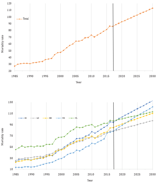
Figure 3 Forecast of Diabetes mortality rate at the national level (top) and based on level of marginalization (bottom) to 2030
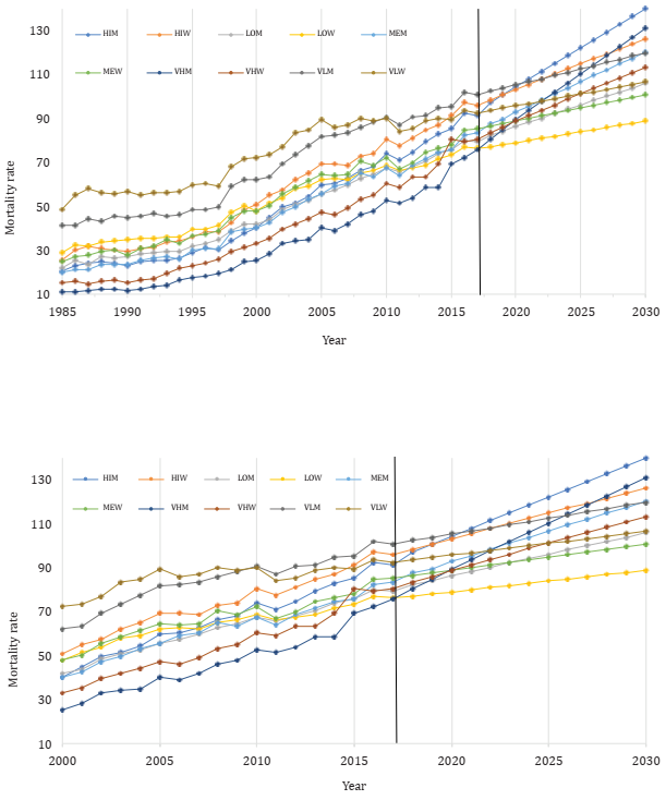
Figure 4 Forecast of Diabetes mortality rate by marginalization and sex (top) and enlarged (bottom) to 2030
Figure 4 presents the observed and forecast rates of mortality separately by marginalization level and sex. In the observed data prior to 2017, women faced a larger burden of mortality related to Diabetes than men (Flores et al., 2016), but again this gap has been shrinking in recent years. In the forecast, many of the ongoing trends in male versus female Diabetes mortality experience a cross over, where men begin to experience higher Diabetes mortality in some sub-areas of the country than women. Similar to what was shown in Figure 3, Figure 4 shows that in areas of High and Very High marginalization, men show forecast rates of Diabetes mortality that cross over female rates and become higher over time.
According to Table 2, the hierarchical forecasts point that the appropriate distribution of the resource allocation should considers mainly the High and Low levels, given that they accumulate more than half of the future deaths by Diabetes in Mexico for the next years. In fact, in each one, the number of male deaths will be greater than female deaths for both levels. The maximum expected of deaths will be for male population at Low level. This scenario highlights the mentioned polarization in Mexico and it also suggest that a preventive health policy should be applied as soon as possible.
Table 2 Percentage of deaths by marginalization and sex: Observed (1985-2017) and forecasted (2018-2030)
| Economic Burden distribution (%) | |||||||||||||||||
|---|---|---|---|---|---|---|---|---|---|---|---|---|---|---|---|---|---|
| Year | Total | Total | |||||||||||||||
| First level | HI | LO | ME | VH | VL | Second level | HIM | HIW | LOM | LOW | MEM | MEW | VHM | VHW | VLM | VLW | |
| 1985 | 100.00 | 20.87 | 27.72 | 13.56 | 5.11 | 32.73 | 100.00 | 9.18 | 11.70 | 11.89 | 15.83 | 6.01 | 7.56 | 2.17 | 2.94 | 14.69 | 18.04 |
| 1986 | 100.00 | 21.94 | 28.56 | 13.45 | 4.78 | 31.28 | 100.00 | 9.48 | 12.46 | 12.43 | 16.14 | 5.88 | 7.57 | 1.97 | 2.81 | 13.16 | 18.12 |
| 1987 | 100.00 | 22.68 | 27.11 | 13.41 | 4.66 | 32.15 | 100.00 | 9.71 | 12.97 | 11.52 | 15.59 | 5.76 | 7.65 | 2.04 | 2.62 | 13.71 | 18.44 |
| 1988 | 100.00 | 21.75 | 29.07 | 14.23 | 4.92 | 30.02 | 100.00 | 9.59 | 12.16 | 12.78 | 16.29 | 6.25 | 7.98 | 2.13 | 2.79 | 12.80 | 17.22 |
| 1989 | 100.00 | 21.37 | 29.16 | 14.38 | 5.04 | 30.06 | 100.00 | 9.44 | 11.93 | 12.64 | 16.52 | 6.30 | 8.08 | 2.13 | 2.91 | 13.26 | 16.80 |
| 1990 | 100.00 | 20.79 | 29.99 | 14.06 | 4.85 | 30.32 | 100.00 | 8.91 | 11.87 | 12.98 | 17.01 | 6.38 | 7.67 | 2.05 | 2.80 | 13.14 | 17.18 |
| 1991 | 100.00 | 21.28 | 30.11 | 14.78 | 4.99 | 28.83 | 100.00 | 9.36 | 11.92 | 13.28 | 16.84 | 6.65 | 8.14 | 2.12 | 2.88 | 12.79 | 16.04 |
| 1992 | 100.00 | 21.16 | 30.02 | 15.02 | 5.08 | 28.72 | 100.00 | 9.29 | 11.87 | 13.36 | 16.65 | 6.72 | 8.30 | 2.22 | 2.86 | 12.82 | 15.89 |
| 1993 | 100.00 | 21.35 | 29.97 | 15.56 | 5.50 | 27.62 | 100.00 | 9.11 | 12.24 | 13.24 | 16.73 | 6.74 | 8.82 | 2.31 | 3.19 | 12.12 | 15.51 |
| 1994 | 100.00 | 21.93 | 29.67 | 14.71 | 6.08 | 27.61 | 100.00 | 9.39 | 12.53 | 13.23 | 16.44 | 6.41 | 8.30 | 2.59 | 3.49 | 12.18 | 15.43 |
| 1995 | 100.00 | 21.55 | 30.41 | 15.37 | 5.97 | 26.70 | 100.00 | 9.46 | 12.09 | 13.47 | 16.94 | 6.84 | 8.53 | 2.58 | 3.39 | 11.68 | 15.01 |
| 1996 | 100.00 | 22.39 | 30.22 | 15.29 | 6.09 | 26.00 | 100.00 | 9.92 | 12.48 | 13.63 | 16.59 | 6.84 | 8.45 | 2.61 | 3.49 | 11.35 | 14.65 |
| 1997 | 100.00 | 21.43 | 31.28 | 15.40 | 6.41 | 25.47 | 100.00 | 9.16 | 12.27 | 14.11 | 17.18 | 6.71 | 8.70 | 2.72 | 3.69 | 11.39 | 14.09 |
| 1998 | 100.00 | 21.09 | 30.78 | 16.01 | 6.29 | 25.83 | 100.00 | 9.20 | 11.89 | 13.72 | 17.06 | 7.22 | 8.79 | 2.59 | 3.70 | 11.76 | 14.07 |
| 1999 | 100.00 | 21.75 | 31.00 | 15.60 | 6.43 | 25.22 | 100.00 | 9.31 | 12.44 | 13.92 | 17.08 | 6.91 | 8.69 | 2.77 | 3.66 | 11.49 | 13.73 |
| 2000 | 100.00 | 22.66 | 30.00 | 15.61 | 6.62 | 25.10 | 100.00 | 9.74 | 12.92 | 13.81 | 16.20 | 6.98 | 8.63 | 2.82 | 3.81 | 11.40 | 13.71 |
| 2001 | 100.00 | 23.49 | 30.09 | 15.48 | 6.81 | 24.13 | 100.00 | 10.25 | 13.23 | 13.64 | 16.44 | 6.95 | 8.54 | 2.95 | 3.86 | 10.97 | 13.16 |
| 2002 | 100.00 | 23.08 | 30.08 | 15.84 | 7.19 | 23.80 | 100.00 | 10.42 | 12.67 | 14.07 | 16.01 | 7.11 | 8.73 | 3.20 | 3.99 | 11.07 | 12.73 |
| 2003 | 100.00 | 23.10 | 30.16 | 15.63 | 7.07 | 24.04 | 100.00 | 10.16 | 12.93 | 13.93 | 16.23 | 7.01 | 8.62 | 3.10 | 3.97 | 11.05 | 12.99 |
| 2004 | 100.00 | 23.32 | 29.79 | 15.94 | 7.06 | 23.90 | 100.00 | 10.31 | 13.01 | 13.83 | 15.96 | 7.23 | 8.71 | 3.03 | 4.03 | 11.22 | 12.68 |
| 2005 | 100.00 | 23.61 | 29.63 | 15.70 | 7.33 | 23.74 | 100.00 | 10.59 | 13.02 | 13.81 | 15.82 | 7.14 | 8.56 | 3.28 | 4.05 | 11.17 | 12.57 |
| 2006 | 100.00 | 23.57 | 30.05 | 16.08 | 7.10 | 23.20 | 100.00 | 10.61 | 12.96 | 14.13 | 15.92 | 7.55 | 8.53 | 3.17 | 3.93 | 11.17 | 12.03 |
| 2007 | 100.00 | 23.37 | 30.12 | 16.05 | 7.48 | 22.99 | 100.00 | 10.76 | 12.61 | 14.51 | 15.61 | 7.57 | 8.48 | 3.36 | 4.12 | 11.05 | 11.94 |
| 2008 | 100.00 | 23.42 | 29.96 | 16.59 | 7.72 | 22.32 | 100.00 | 10.77 | 12.65 | 14.43 | 15.53 | 7.82 | 8.78 | 3.48 | 4.24 | 10.71 | 11.61 |
| 2009 | 100.00 | 23.61 | 30.23 | 16.04 | 7.93 | 22.19 | 100.00 | 10.94 | 12.67 | 14.67 | 15.56 | 7.56 | 8.48 | 3.59 | 4.34 | 10.86 | 11.33 |
| 2010 | 100.00 | 24.29 | 30.03 | 16.11 | 8.25 | 21.32 | 100.00 | 11.28 | 13.01 | 14.69 | 15.33 | 7.63 | 8.47 | 3.73 | 4.52 | 10.51 | 10.82 |
| 2011 | 100.00 | 24.37 | 30.43 | 15.78 | 8.42 | 21.00 | 100.00 | 11.33 | 13.04 | 14.89 | 15.54 | 7.59 | 8.20 | 3.82 | 4.60 | 10.48 | 10.52 |
| 2012 | 100.00 | 24.56 | 29.98 | 16.14 | 8.59 | 20.73 | 100.00 | 11.43 | 13.13 | 14.84 | 15.15 | 7.87 | 8.27 | 3.82 | 4.76 | 10.51 | 10.21 |
| 2013 | 100.00 | 24.88 | 29.68 | 16.42 | 8.62 | 20.39 | 100.00 | 11.67 | 13.21 | 14.78 | 14.91 | 7.92 | 8.51 | 4.02 | 4.61 | 10.11 | 10.28 |
| 2014 | 100.00 | 24.86 | 29.98 | 16.39 | 8.71 | 20.06 | 100.00 | 11.78 | 13.08 | 14.96 | 15.02 | 7.96 | 8.43 | 3.86 | 4.84 | 10.12 | 9.95 |
| 2015 | 100.00 | 24.92 | 29.75 | 16.16 | 9.83 | 19.33 | 100.00 | 11.69 | 13.24 | 14.86 | 14.90 | 7.82 | 8.34 | 4.41 | 5.43 | 9.76 | 9.57 |
| 2016 | 100.00 | 25.27 | 29.52 | 16.60 | 9.37 | 19.24 | 100.00 | 11.95 | 13.32 | 14.84 | 14.68 | 8.04 | 8.56 | 4.33 | 5.04 | 9.83 | 9.41 |
| 2017 | 100.00 | 25.06 | 29.38 | 16.81 | 9.68 | 19.06 | 100.00 | 11.85 | 13.21 | 14.76 | 14.62 | 8.19 | 8.63 | 4.54 | 5.14 | 9.76 | 9.30 |
| 2018 | 100.00 | 25.34 | 29.29 | 16.84 | 9.83 | 18.70 | 100.00 | 12.22 | 13.13 | 14.89 | 14.40 | 8.34 | 8.50 | 4.68 | 5.15 | 9.59 | 9.11 |
| 2019 | 100.00 | 25.50 | 29.20 | 16.81 | 10.01 | 18.47 | 100.00 | 12.38 | 13.13 | 14.93 | 14.27 | 8.37 | 8.44 | 4.82 | 5.19 | 9.48 | 8.99 |
| 2020 | 100.00 | 25.63 | 29.10 | 16.85 | 10.17 | 18.24 | 100.00 | 12.52 | 13.11 | 14.96 | 14.14 | 8.48 | 8.37 | 4.95 | 5.22 | 9.37 | 8.87 |
| 2021 | 100.00 | 25.76 | 29.02 | 16.86 | 10.33 | 18.03 | 100.00 | 12.65 | 13.10 | 15.00 | 14.02 | 8.54 | 8.31 | 5.08 | 5.26 | 9.28 | 8.75 |
| 2022 | 100.00 | 25.88 | 28.94 | 16.88 | 10.48 | 17.83 | 100.00 | 12.78 | 13.09 | 15.03 | 13.91 | 8.62 | 8.25 | 5.19 | 5.28 | 9.18 | 8.65 |
| 2023 | 100.00 | 25.99 | 28.86 | 16.89 | 10.62 | 17.64 | 100.00 | 12.90 | 13.09 | 15.06 | 13.81 | 8.69 | 8.20 | 5.30 | 5.31 | 9.10 | 8.55 |
| 2024 | 100.00 | 26.09 | 28.79 | 16.90 | 10.75 | 17.47 | 100.00 | 13.01 | 13.08 | 15.08 | 13.71 | 8.75 | 8.15 | 5.41 | 5.34 | 9.01 | 8.45 |
| 2025 | 100.00 | 26.19 | 28.72 | 16.91 | 10.87 | 17.30 | 100.00 | 13.12 | 13.07 | 15.11 | 13.61 | 8.81 | 8.10 | 5.50 | 5.37 | 8.94 | 8.36 |
| 2026 | 100.00 | 26.29 | 28.66 | 16.92 | 10.99 | 17.14 | 100.00 | 13.22 | 13.07 | 15.13 | 13.53 | 8.87 | 8.05 | 5.60 | 5.39 | 8.86 | 8.28 |
| 2027 | 100.00 | 26.38 | 28.60 | 16.93 | 11.10 | 16.99 | 100.00 | 13.32 | 13.06 | 15.16 | 13.44 | 8.92 | 8.01 | 5.68 | 5.41 | 8.79 | 8.20 |
| 2028 | 100.00 | 26.46 | 28.54 | 16.95 | 11.20 | 16.85 | 100.00 | 13.41 | 13.05 | 15.18 | 13.36 | 8.98 | 7.97 | 5.77 | 5.43 | 8.73 | 8.12 |
| 2029 | 100.00 | 26.54 | 28.48 | 16.95 | 11.30 | 16.71 | 100.00 | 13.50 | 13.05 | 15.20 | 13.29 | 9.02 | 7.93 | 5.85 | 5.46 | 8.66 | 8.05 |
| 2030 | 100.00 | 26.62 | 28.43 | 16.96 | 11.40 | 16.59 | 100.00 | 13.58 | 13.04 | 15.22 | 13.21 | 9.07 | 7.89 | 5.92 | 5.47 | 8.60 | 7.98 |
It is also important to recognize that the Medium and Very Low levels will jointly concentrate 1 of every 3 deaths from Diabetes in Mexico (see Table 2). It is also observed that the deaths per sex for both levels will be greater for male population. The smallest resource is required for the Very High level where the poverty and its consequences are their main characteristics. In other words, there is not a direct relationship among the marginalization and the expected percentage of deaths by Diabetes for the mexican case.
Conclusion
This analysis presents results of an analysis of hierarchical forecasts applied to the problem of distribution of resources to address the burden that Diabetes mortality is expected for Mexico by 2030. Overall, the forecasts estimated here show significant differences based on levels of marginalization and sex. Likewise, the gaps between men and women are notorious as well as between the levels of marginalization. Thereby, there is enough evidence that is not a good idea to consider a uniform distribution to face the economic burden caused by the Diabetes.
The hierarchical forecasts show that if the current trends continue, there will be a divergence by marginalization and sex in mortality in Mexico. Even worse, these forecasts indicate that the rates will increase the most simultaneously at high income level and some poor areas of the country. Through this statistical tool, it was possible to show not only the long-term trends in Diabetes mortality, but how the trends vary among areas of the country and by subpopulations.
The phenomenon presents notable differences by marginalization and sex; in fact, the increase in the mortality rate is clearly differentiated. This suggest that it could be necessary to implement preventive and specific health policies based on geographic region. It is also evident that the current preventive health policies need be rethought to reduce mortality from Diabetes in Mexico.

